Every problem in regreg is put in composite form,
with smooth (its gradient is Lipschitz) and convex with a cheap proximal map
The main solver is FISTA, the accelerated proximal gradient method of Beck
and Teboulle (2009). Each iteration takes a gradient step on from an
extrapolated point and then applies the proximal map of . This page
describes the problem containers and solver options, how to plug in your
own problem, and the alternatives for problems that do not fit this
pattern directly: dual solves for container, ADMM, TFOCS/NESTA-style
smoothing, and a proximal quasi-Newton method.
import time
import numpy as np
import matplotlib.pyplot as plt
from scipy.optimize import linprog, lsq_linear

import regreg.api as rrsimple_problem: one smooth part, one atom
rr.simple_problem(loss, atom) pairs a smooth loss with a single atom whose
proximal map is known exactly. Its solve method runs FISTA and returns
the solution; keyword arguments go to FISTA.fit:
tol(default1e-5): stop when the relative change in objective (or, withcoef_stop=True, in coefficients) falls belowtol;min_its(default 5) andmax_its(default 10000);FISTA(defaultTrue): use Nesterov momentum;Falsegives plain proximal gradient descent (ISTA);start_step(default 1): the initial step size for backtracking;restart(default never): reset momentum everyrestartiterations;monotonicity_restart(defaultTrue): reset momentum whenever the objective increases (adaptive restart);coef_stop(defaultFalse): use the coefficient-change criterion;debug: print the objective, step size and relative change at each iteration.
The step size is chosen by backtracking: it is decreased by a factor
1.1 until the usual quadratic upper bound on holds, and tentatively
increased every 100 iterations. After solve, the history of objective
values is in problem.solver_results and the final step in
problem.final_step. Because the backtracking condition is only checked
along the iterates, the accepted step reflects the local curvature of
and can be much larger than , where is the global Lipschitz
constant of . In the example below is dominated
by the factor shared by all columns, and the final step is about ten times
.
rng = np.random.default_rng(0)
n, p = 100, 400
X = 0.3 * rng.standard_normal((n, p)) + rng.standard_normal((n, 1))  # correlated columns
beta = np.zeros(p)
beta[:10] = 3
Y = X @ beta + rng.standard_normal(n)
lam = 0.05 * np.abs(X.T @ Y).max()

def lasso():
    return rr.simple_problem(rr.squared_error(X, Y), rr.l1norm(p, lagrange=lam))

problem = lasso()
beta_hat = problem.solve(tol=1e-10)
print('iterations:', len(problem.solver_results))
print('final step: %.3g   1/L: %.3g' % (problem.final_step, 1 / np.linalg.norm(X, 2)**2))
print('nonzero coefficients:', (beta_hat != 0).sum())
iterations: 545
final step: 0.000276 1/L: 2.58e-05
nonzero coefficients: 35
Using FISTA directly
rr.FISTA(problem) creates the solver; fit takes the same arguments as
above and returns the vector of objective values, one per iteration. The
solution is written into problem.coefs (FISTA modifies the problem’s
coefficients in place, so a second fit warm starts from the previous
solution).
Momentum matters. With correlated columns the problem is badly conditioned and ISTA converges at rate , against for FISTA. Without adaptive restart FISTA’s objective is not monotone and it oscillates; restarting the momentum whenever the objective increases (the default) removes the oscillation and typically converges fastest.
f_star = lasso().objective(lasso().solve(tol=1e-15, min_its=20000, max_its=20000))

histories = {}
for label, kwargs in [('FISTA (default)', {}),
                      ('FISTA, no restart', {'monotonicity_restart': False}),
                      ('ISTA', {'FISTA': False})]:
    solver = rr.FISTA(lasso())
    histories[label] = solver.fit(tol=1e-12, max_its=2000, **kwargs)
    print('%-18s iterations: %4d   f - f*: %.1e' % (label, len(histories[label]),
                                                    histories[label][-1] - f_star))

assert histories['FISTA (default)'][-1] - f_star < 1e-6 * f_star
FISTA (default) iterations: 654 f - f*: -8.4e-07
FISTA, no restart iterations: 2000 f - f*: 1.7e-02
ISTA iterations: 2000 f - f*: 3.4e+00
fig, ax = plt.subplots(figsize=(7, 4))
for label, hist in histories.items():
    ax.semilogy(np.maximum(hist - f_star, 1e-12) / f_star, label=label)
ax.set_xlabel('iteration')
ax.set_ylabel(r'$(F(\beta_k) - F^*) / F^*$')
ax.legend();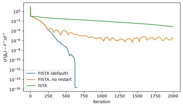
Fixed step size
Backtracking costs extra evaluations of . If the Lipschitz constant
is known, set solver.perform_backtrack = False and give the problem a
lipschitz attribute; FISTA then uses step throughout.
rr.power_L(X) estimates , which is for least squares.
For this problem the global constant is pessimistic, and the fixed step
needs more iterations than backtracking.
problem = lasso()
problem.lipschitz = rr.power_L(X)
solver = rr.FISTA(problem)
solver.perform_backtrack = False
hist = solver.fit(tol=1e-12)
print('iterations:', len(hist), '  f - f*: %.1e' % (hist[-1] - f_star))
assert hist[-1] - f_star < 1e-6 * f_star
iterations: 1475 f - f*: 1.2e-05
Defining your own problem: the composite interface
FISTA only needs four things from a problem: a coefs array (the starting
point, overwritten with the solution), smooth_objective(x, mode) returning
the value (mode='func'), gradient ('grad') or both ('both') of ,
nonsmooth_objective(x) returning , and proximal(q). The argument
q of proximal is an rr.identity_quadratic, the function
, and
proximal must return the minimizer of . Its
attribute q.true_center is , so the proximal map is
evaluated at q.true_center with step where is q.coef.
Subclassing rr.composite provides coefs, objective and the plumbing.
As an example, here is least squares under box constraints
, whose proximal map is clipping, compared with
scipy.optimize.lsq_linear.
class box_least_squares(rr.composite):

    def __init__(self, X, Y, lower, upper):
        self.X, self.Y, self.lower, self.upper = X, Y, lower, upper
        rr.composite.__init__(self, X.shape[1])

    def smooth_objective(self, beta, mode='both', check_feasibility=False):
        resid = self.X @ beta - self.Y
        f, g = 0.5 * resid @ resid, self.X.T @ resid
        return {'func': f, 'grad': g, 'both': (f, g)}[mode]

    def nonsmooth_objective(self, beta, check_feasibility=False):
        inside = np.all((beta >= self.lower - 1e-10) & (beta <= self.upper + 1e-10))
        return 0. if inside else np.inf

    def proximal(self, q, prox_control=None):
        return np.clip(q.true_center, self.lower, self.upper)

rng = np.random.default_rng(1)
Xb = rng.standard_normal((50, 10))
Yb = 3 * rng.standard_normal(50)

box = box_least_squares(Xb, Yb, -0.2, 0.2)
rr.FISTA(box).fit(tol=1e-14, min_its=100)
reference = lsq_linear(Xb, Yb, bounds=(-0.2, 0.2), tol=1e-12).x

print(np.round(box.coefs, 3))
print('max |regreg - lsq_linear|:', np.abs(box.coefs - reference).max())
np.testing.assert_allclose(box.coefs, reference, atol=1e-7)
[ 0.2 -0.082 -0.2 0.196 0.2 -0.085 0.2 0.2 -0.2 0.2 ]
max |regreg - lsq_linear|: 8.318296051967877e-11
regreg’s own atoms and smooth losses implement the same interface (with
the quadratic term handled for you), so they can be mixed with
hand-written pieces: for instance rr.simple_problem(my_smooth, atom)
works for any object with smooth_objective and coefs.
container: several atoms, solved through the dual
rr.container(loss, atom_1, ..., atom_k) minimizes
where the atoms are
possibly composed with affine maps (see
constraints and linear transforms). The proximal map of
the sum has no closed form, so at every FISTA step the container solves the
dual of the proximal problem,
by an inner FISTA run (with fixed step from power_L of the stacked
), and recovers . The conjugates
are again atoms with exact proximal maps. The inner solver
can be controlled by passing prox_control, a dictionary of fit
arguments (defaults tol=1e-14, max_its=5000), to solve or fit.
Because the inner solve is iterative, the outer solve is accurate only to
roughly the precision of the inner one.
Below is a generalized lasso, with a random .
rng = np.random.default_rng(2)
n, p, m = 200, 100, 30
X = rng.standard_normal((n, p))
Y = X @ np.r_[3 * np.ones(10), np.zeros(p - 10)] + rng.standard_normal(n)
D = rng.standard_normal((m, p))
lam = 0.2 * np.abs(X.T @ Y).max()

genlasso = rr.container(rr.squared_error(X, Y), rr.l1norm.linear(D, lagrange=lam))
tic = time.time()
beta_container = genlasso.solve(tol=1e-12)
print('container: %.2fs, objective %.6f' % (time.time() - tic,
                                            genlasso.objective(beta_container)))
container: 5.53s, objective 2317.844370
ADMM
The alternating direction method of multipliers handles the same generalized problem by splitting and alternating
regreg.problems.admm.admm_problem(loss, atom, D, rho) implements this; the
-update is a smooth problem solved by FISTA (with arguments from
fit_args), and solve(niter) runs a fixed number of iterations. The
primal iterate is loss_coefs. Each iteration is cheap but ADMM converges
slowly to high accuracy; here 200 iterations agree with the container to
about 10-5.
from regreg.problems.admm import admm_problem

admm = admm_problem(rr.squared_error(X, Y), rr.l1norm(m, lagrange=lam), D, 1.)
tic = time.time()
admm.solve(niter=200)
beta_admm = admm.loss_coefs
print('ADMM: %.2fs, objective %.6f' % (time.time() - tic, genlasso.objective(beta_admm)))
print('max |ADMM - container|:', np.abs(beta_admm - beta_container).max())
np.testing.assert_allclose(beta_admm, beta_container, atol=1e-3)
ADMM: 1.71s, objective 2317.844436
max |ADMM - container|: 1.3045302673653225e-06
Smoothing: TFOCS and NESTA
Some problems have no smooth part at all. Two examples are basis pursuit (Chen, Donoho and Saunders, 1998),
and the Dantzig selector (Candès and Tao, 2007), subject to . Both have the form
where and have simple proximal maps but neither is smooth: for basis pursuit , , and is the indicator of . Two ways of making such a problem amenable to FISTA are to smooth the dual (TFOCS) or to smooth (NESTA). In both, the smoothing term has a center that is moved from one outer iteration to the next, so that the iterates converge to a solution of the original problem rather than of a smoothed one.
TFOCS: smoothing the dual
Add a proximal term to : with , consider (Becker, Candès and Grant, 2011). Writing and exchanging the min and the max gives the dual problem
Because is -strongly convex, its conjugate is differentiable, with gradient
which is Lipschitz with constant (Nesterov, 2005). So the
dual is a smooth function, with Lipschitz constant ,
plus , which has a proximal map: a simple_problem for FISTA. Its
solution gives the primal solution
of the regularized problem.
The outer loop sets and repeats. This is the
proximal point method (Rockafellar, 1976) applied to ,
so for any fixed the iterates converge to a solution of the
original problem; rr.tfocs also extrapolates the center, as in Güler’s
(1992) accelerated proximal point method. The value of trades
the two loops against each other. A small makes each outer
step nearly a full step towards the solution, so few outer iterations are
needed, but makes the inner problem worse conditioned (Lipschitz constant
). A large does the reverse. It changes how
long the solve takes, not the accuracy of the answer, which is set by the
inner tolerance tol and the outer tolerance coef_tol.
rr.tfocs(h, transform, k_conjugate, epsilon=[...]) runs this scheme, with
at most one outer iteration per entry of epsilon. The pair
(transform, k_conjugate) is the dual attribute of the composed atom
: transform is and
k_conjugate is . For basis pursuit we check the result against a
linear-programming solve, for several values of .
rng = np.random.default_rng(3)
n, p = 100, 300
X = rng.standard_normal((n, p))
beta = np.zeros(p)
beta[:8] = np.arange(8) + 1
Y = X @ beta                           # noiseless

# basis pursuit as a linear program in (beta^+, beta^-)
lp = linprog(np.ones(2 * p), A_eq=np.hstack([X, -X]), b_eq=Y, bounds=(0, None))
beta_lp = lp.x[:p] - lp.x[p:]

for eps in [10., 1., 0.1]:
    l1 = rr.l1norm(p, lagrange=1)
    transform, zero = rr.zero_constraint.affine(X, -Y).dual
    tic = time.time()
    beta_tfocs, u_tfocs = rr.tfocs(l1, transform, zero, epsilon=[eps] * 100)
    print('eps %-5g  %.2fs  max |tfocs - LP| = %.1e  max |X beta - Y| = %.1e'
          % (eps, time.time() - tic, np.abs(beta_tfocs - beta_lp).max(),
             np.abs(X @ beta_tfocs - Y).max()))
    np.testing.assert_allclose(beta_tfocs, beta_lp, atol=1e-6)
eps 10 0.45s max |tfocs - LP| = 3.9e-08 max |X beta - Y| = 1.1e-07
eps 1      0.29s  max |tfocs - LP| = 2.4e-08  max |X beta - Y| = 1.5e-07
eps 0.1    0.10s  max |tfocs - LP| = 3.1e-09  max |X beta - Y| = 1.2e-08
The Dantzig selector’s constraint is
rr.supnorm.affine(X.T @ X, -X.T @ Y, bound=delta), so here
and the inner problem has Lipschitz constant , much
larger than for basis pursuit (printed below). The inner problems are
therefore slower; for harder instances (a smaller , more active
constraints) a larger or more outer iterations may be needed.
Y_noisy = Y + 0.5 * rng.standard_normal(n)
G, g = X.T @ X, X.T @ Y_noisy
delta = 0.5 * np.sqrt(2 * np.log(p) * n)

transform, k_conjugate = rr.supnorm.affine(G, -g, bound=delta).dual
print('||X^T X||^2 = %.3g,  ||X||^2 = %.3g' % (np.linalg.norm(G, 2)**2, np.linalg.norm(X, 2)**2))
tic = time.time()
beta_ds, _ = rr.tfocs(rr.l1norm(p, lagrange=1), transform, k_conjugate, epsilon=[1.] * 50)
print('Dantzig selector: %.2fs' % (time.time() - tic))

lp = linprog(np.ones(2 * p),
             A_ub=np.vstack([np.hstack([G, -G]), np.hstack([-G, G])]),
             b_ub=np.r_[delta + g, delta - g], bounds=(0, None))
beta_ds_lp = lp.x[:p] - lp.x[p:]
print('||X^T(Y - X beta)||_inf / delta: %.5f' % (np.abs(g - G @ beta_ds).max() / delta))
print('l1 norm: tfocs %.5f   LP %.5f' % (np.abs(beta_ds).sum(), np.abs(beta_ds_lp).sum()))
print('max |tfocs - LP|:', np.abs(beta_ds - beta_ds_lp).max())
np.testing.assert_allclose(beta_ds, beta_ds_lp, atol=1e-5)
||X^T X||^2 = 5.06e+05, ||X||^2 = 711
Dantzig selector: 0.88s
||X^T(Y - X beta)||_inf / delta: 1.00000
l1 norm: tfocs 34.61098   LP 34.61098
max |tfocs - LP|: 1.3115681962716508e-07
NESTA: smoothing the constraint
The other option keeps the proximal map of and smooths instead,
by adding a quadratic to its conjugate (the atom method smoothed):
is smooth with Lipschitz constant (Nesterov,
2005), so is a smooth function plus an
atom, a simple_problem. For an equality constraint , and
the augmented Lagrangian with multiplier and penalty .
The outer loop sets , the
method of multipliers (Hestenes, 1969; Powell, 1969), which is the proximal
point method applied to the dual (Rockafellar, 1976). As for TFOCS, the
iterates converge for any fixed , and affects the
speed only. NESTA itself (Becker, Bobin and Candès, 2011) smooths
rather than the constraint, with continuation in the smoothing parameter;
rr.nesta is an accelerated augmented-Lagrangian method in the same
spirit, and also allows an extra smooth term.
rr.nesta(smooth, h, k_atom, epsilon=[...]) takes the composed atom
itself, and smooth (which may be None) is an additional smooth term in
the objective.
for eps in [10., 1., 0.1]:
    tic = time.time()
    beta_nesta, u_nesta = rr.nesta(None, rr.l1norm(p, lagrange=1),
                                   rr.zero_constraint.affine(X, -Y), epsilon=[eps] * 100)
    print('eps %-5g  %.2fs  max |nesta - LP| = %.1e'
          % (eps, time.time() - tic, np.abs(beta_nesta - beta_lp).max()))
    np.testing.assert_allclose(beta_nesta, beta_lp, atol=1e-5)
eps 10 0.06s max |nesta - LP| = 1.5e-06
eps 1 0.09s max |nesta - LP| = 9.1e-07
eps 0.1 0.19s max |nesta - LP| = 8.3e-08
References
Beck, A. and Teboulle, M. (2009). A fast iterative shrinkage-thresholding algorithm for linear inverse problems. SIAM Journal on Imaging Sciences, 2(1), 183–202.
Becker, S., Bobin, J. and Candès, E. J. (2011). NESTA: a fast and accurate first-order method for sparse recovery. SIAM Journal on Imaging Sciences, 4(1), 1–39.
Becker, S., Candès, E. J. and Grant, M. (2011). Templates for convex cone problems with applications to sparse signal recovery. Mathematical Programming Computation, 3(3), 165–218.
Candès, E. and Tao, T. (2007). The Dantzig selector: statistical estimation when is much larger than . The Annals of Statistics, 35(6), 2313–2351.
Chen, S. S., Donoho, D. L. and Saunders, M. A. (1998). Atomic decomposition by basis pursuit. SIAM Journal on Scientific Computing, 20(1), 33–61.
Güler, O. (1992). New proximal point algorithms for convex minimization. SIAM Journal on Optimization, 2(4), 649–664.
Hestenes, M. R. (1969). Multiplier and gradient methods. Journal of Optimization Theory and Applications, 4(5), 303–320.
Nesterov, Yu. (2005). Smooth minimization of non-smooth functions. Mathematical Programming, 103(1), 127–152.
Powell, M. J. D. (1969). A method for nonlinear constraints in minimization problems. In R. Fletcher (ed.), Optimization, 283–298. Academic Press.
Rockafellar, R. T. (1976). Augmented Lagrangians and applications of the proximal point algorithm in convex programming. Mathematics of Operations Research, 1(2), 97–116.
Proximal quasi-Newton
For smooth losses with strong curvature, such as logistic regression,
proximal Newton methods (Lee, Sun and Saunders, 2014) take fewer, more
expensive steps. At each step they minimize the quadratic model of
plus , ,
and then line search along . regreg.problems.newton.quasi_newton
does this with BFGS updates of , starting from a user-supplied
initial_hessian. The quadratic subproblems are solved by FISTA, and the
keyword arguments of solve are passed to that inner solver.
from regreg.problems.newton import quasi_newton

rng = np.random.default_rng(4)
n, p = 500, 50
X = rng.standard_normal((n, p))
eta = X @ np.r_[np.ones(5), np.zeros(p - 5)]
Y = rng.binomial(1, 1 / (1 + np.exp(-eta)))
lam = 0.1 * np.abs(X.T @ (Y - Y.mean())).max()

fista_problem = rr.simple_problem(rr.glm.logistic(X, Y), rr.l1norm(p, lagrange=lam))
beta_fista = fista_problem.solve(tol=1e-12, min_its=50)

qn = quasi_newton(rr.glm.logistic(X, Y), rr.l1norm(p, lagrange=lam),
                  initial_hessian=X.T @ X / 4)
beta_qn = qn.solve(niter=30, tol=1e-12)
print('quasi-Newton steps:', len(qn.solver_results) - 1)
print('max |quasi-Newton - FISTA|:', np.abs(beta_qn - beta_fista).max())
np.testing.assert_allclose(beta_qn, beta_fista, atol=1e-5)
quasi-Newton steps: 11
max |quasi-Newton - FISTA|: 6.841502411623207e-07
Which solver?
For a smooth loss plus one atom (possibly separable), use
simple_problem, whose proximal step is exact. Add atoms composed with
linear maps through container, which is convenient but solves a dual
problem at every step. ADMM is an alternative when the -update is
cheap or can be reused. For problems with no smooth part, such as
constrained minimization, use TFOCS- or NESTA-style smoothing.