The regreg.paths subpackage computes solutions of penalized problems of the form
over a decreasing sequence . Here is a
loss of the linear predictor (Gaussian, logistic, probit, cloglog, Poisson, Cox, Huber, ...),
is a (weighted) , group lasso or sparse group lasso penalty,
is the elastic net mixing parameter and are the ridge weights
(elastic_net_param). With (the default) this is the lasso, group lasso, etc.
A path computation has three ingredients:
a path object, which describes the loss, design and penalty. These live in
regreg.paths.lasso,group_lasso,sparse_group_lasso,sparse_group_blockandmixed_lasso, and are built by module-level constructors such aslasso.gaussian(X, Y, weights)orgroup_lasso.logistic(X, Y, groups, weights=...);a sequence of Lagrange parameters, usually from
default_lagrange_sequence;a driver:
strong_rulesorwarm_start(inregreg.paths) orbasil(inregreg.paths.basil).
import numpy as np
import matplotlib.pyplot as plt

import regreg.api as rr
from regreg.paths import (lasso,
                          group_lasso,
                          strong_rules,
                          warm_start,
                          default_lagrange_sequence)
from regreg.paths.basil import basil
from regreg.paths.cross_validate import cross_validate
Note the import locations: regreg.paths.basil and regreg.paths.cross_validate are
submodules, so the functions must be imported from them.
A lasso path
We simulate a sparse linear model with five nonzero coefficients.
rng = np.random.default_rng(0)
n, p = 200, 30
X = rng.standard_normal((n, p))
beta = np.zeros(p)
beta[:5] = [3, -2, 1.5, 1, -0.5]
Y = X @ beta + rng.standard_normal(n)

path = lasso.gaussian(X, Y, np.ones(p))   # weights: one l1 weight per feature
The path object stores the solution at (the “null” solution, here
) as path.solution, and the gradient of the loss there as
path.grad_solution. The smallest for which the null solution is optimal,
, is the dual norm of this gradient; for the lasso with squared error loss
it is .
default_lagrange_sequence returns nstep log-spaced values from down to
lagrange_proportion .
lagrange = default_lagrange_sequence(path.penalty,
                                     path.grad_solution,
                                     lagrange_proportion=0.01,
                                     nstep=30)
np.testing.assert_allclose(lagrange[0], np.fabs(X.T @ Y).max())
lagrange[:3], lagrange[-1] / lagrange[0]
(array([631.084251 , 538.42079512, 459.36331347]),
np.float64(0.010000000000000004))Every driver takes the path object, the sequence and the initial (solution, gradient)
pair at lagrange[0]. strong_rules returns a dictionary; its 'beta' entry has one
row per value of .
initial = (path.solution.copy(), path.grad_solution.copy())
sr = strong_rules(path, lagrange, initial, inner_tol=1e-10)
B_sr = sr['beta']
B_sr.shape
(30, 30)fig, ax = plt.subplots(figsize=(7, 4.5))
loglam = np.log(lagrange)
for j in range(5, p):
ax.plot(loglam, B_sr[:, j], color='0.7', lw=1)
colors = ['#1f77b4', '#ff7f0e', '#2ca02c', '#d62728', '#9467bd']
for j in range(5):
ax.plot(loglam, B_sr[:, j], color=colors[j], lw=2, label=r'$\beta_{%d}=%g$' % (j + 1, beta[j]))
ax.axhline(0, color='k', lw=0.5)
ax.invert_xaxis()
ax.set_xlabel(r'$\log \lambda$')
ax.set_ylabel('coefficient')
ax.set_title('Lasso path (true signals in color, nulls in gray)')
ax.legend(frameon=False, fontsize=9);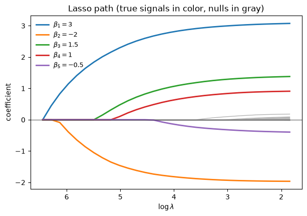
Three drivers, one path
warm_startsolves the full problem at each , starting from the previous solution. It is the simplest and the reference implementation.strong_rulessolves each problem on a small working set chosen by the sequential strong rule of Tibshirani et al. (2012), then checks the KKT conditions on all variables and enlarges the working set until they hold.basil(batch screening iterative lasso) adds thestep_nvarlargest KKT violators at a time and solvesstep_lagrangevalues of per batch.
All three should give the same path. We also compare with a direct solve of each problem
using rr.simple_problem.
path = lasso.gaussian(X, Y, np.ones(p))
B_ws = warm_start(path, lagrange, initial, inner_tol=1e-10)['beta']

path = lasso.gaussian(X, Y, np.ones(p))
B_basil = basil(path, lagrange, initial, inner_tol=1e-10, step_nvar=10, step_lagrange=5)

loss = rr.squared_error(X, Y)
B_direct = np.array([rr.simple_problem(loss, rr.l1norm(p, lagrange=lam)).solve(tol=1e-13, min_its=500)
                     for lam in lagrange])

for name, B in [('strong_rules', B_sr), ('warm_start', B_ws), ('basil', B_basil)]:
    print('%-13s max |beta - direct| = %.2e' % (name, np.fabs(B - B_direct).max()))
print('max |strong_rules - warm_start| = %.2e' % np.fabs(B_sr - B_ws).max())
print('max |basil - warm_start|        = %.2e' % np.fabs(B_basil - B_ws).max())
strong_rules max |beta - direct| = 2.50e-09
warm_start max |beta - direct| = 4.80e-05
basil max |beta - direct| = 4.09e-05
max |strong_rules - warm_start| = 4.80e-05
max |basil - warm_start| = 4.83e-05
Before a step is accepted, the drivers check the KKT conditions on all variables. An
inactive variable fails the check when , and then joins the working set. The tolerance is
kkt_tol, with default 1e-6. It is an attribute of the path object (path.kkt_tol), and the drivers
also take it as an argument. A looser value saves little time and can leave a variable
that is just about to enter at zero for a step. Earlier versions used 1%, which
gave errors of order 10-3 near entry points
(gh-99). The KKT checks of the active
variables (check_active=True) use their own, looser, tolerance, as they depend on how
accurately each subproblem is solved.
strong_rules agrees with the direct solves to the solver tolerance at every
. The 10-5-level errors of warm_start and basil come from the
stopping rule of their solves, which is not as strict as inner_tol suggests.
print(np.array2string(np.fabs(B_sr - B_direct).max(1), precision=1))[0.0e+00 2.7e-10 2.2e-10 1.1e-10 1.0e-10 2.8e-10 4.9e-11 1.2e-10 3.6e-10
2.1e-10 3.6e-10 7.6e-10 6.4e-10 4.1e-11 5.5e-10 5.3e-10 1.3e-09 1.5e-10
3.0e-10 5.1e-10 2.8e-11 2.6e-10 1.5e-10 7.4e-11 3.6e-10 1.1e-10 2.3e-10
2.5e-09 3.7e-10 2.2e-09]
np.testing.assert_allclose(B_sr, B_direct, atol=1e-6)
np.testing.assert_allclose(B_basil, B_direct, atol=5e-4)
np.testing.assert_allclose(B_ws, B_direct, atol=5e-4)
Elastic net
Set alpha < 1 for the elastic net. Pass the same alpha to default_lagrange_sequence,
which divides the sequence by so that it still starts at the first
where a variable enters.
enet = lasso.gaussian(X, Y, np.ones(p), alpha=0.5)
lagrange_enet = default_lagrange_sequence(enet.penalty, enet.grad_solution,
                                          lagrange_proportion=0.05, nstep=15, alpha=enet.alpha)
init_enet = (enet.solution.copy(), enet.grad_solution.copy())
B_enet = strong_rules(enet, lagrange_enet, init_enet, inner_tol=1e-10)['beta']

# direct solve at the smallest lambda: 0.5 * ||Y - X b||^2 + lam * (0.5 ||b||_1 + 0.25 ||b||_2^2)
lam = lagrange_enet[-1]
ridge = rr.identity_quadratic(lam * 0.5, 0, 0, 0)
direct = rr.simple_problem(loss, rr.l1norm(p, lagrange=0.5 * lam)).solve(ridge, tol=1e-13, min_its=500)
print('elastic net, max |path - direct| = %.2e' % np.fabs(B_enet[-1] - direct).max())
np.testing.assert_allclose(B_enet[-1], direct, atol=1e-6)
elastic net, max |path - direct| = 5.55e-10
Unpenalized variables: a group lasso path
Variables with penalty weight 0 are unpenalized. They are fitted in the null solution (by solving the problem with only those variables) and kept in every subproblem. Here the first group of three variables is unpenalized; the other five groups get the usual weight .
rng = np.random.default_rng(1)
n = 150
groups = np.repeat(np.arange(6), 3)
p = groups.shape[0]
X = rng.standard_normal((n, p))
beta = np.zeros(p)
beta[:3] = 1
beta[3:6] = [2, -1, 0.5]
Y = X @ beta + rng.standard_normal(n)

weights = {g: np.sqrt(3) for g in range(1, 6)}
weights[0] = 0.

# with unpenalized variables, give them ridge weight 0 (otherwise a warning is issued)
enet_param = (groups != 0).astype(float)
gpath = group_lasso.gaussian(X, Y, groups, weights=weights, elastic_net_param=enet_param)
The null solution is the least squares fit on the unpenalized group:
ols = np.linalg.lstsq(X[:, :3], Y, rcond=None)[0]
print(gpath.solution[:3], ols)
np.testing.assert_allclose(gpath.solution[:3], ols, atol=1e-3)
[1.11616196 1.23184926 0.78500781] [1.11615923 1.23185397 0.78499189]
lagrange_g = default_lagrange_sequence(gpath.penalty, gpath.grad_solution,
                                       lagrange_proportion=0.02, nstep=20)
B_g = strong_rules(gpath, lagrange_g, (gpath.solution.copy(), gpath.grad_solution.copy()),
                   inner_tol=1e-10)['beta']

# which groups are active at each lambda?
active = np.array([[np.any(b[groups == g] != 0) for g in range(6)] for b in B_g])
print(active.astype(int)[::4])

pen = rr.group_lasso(groups, weights=weights, lagrange=lagrange_g[-1])
direct = rr.simple_problem(rr.squared_error(X, Y), pen).solve(tol=1e-13, min_its=500)
print('group lasso, max |path - direct| = %.2e' % np.fabs(B_g[-1] - direct).max())
np.testing.assert_allclose(B_g[-1], direct, atol=1e-6)
[[1 0 0 0 0 0]
[1 1 0 0 0 0]
[1 1 0 0 0 0]
[1 1 0 0 0 0]
[1 1 0 0 0 0]]
group lasso, max |path - direct| = 7.88e-11
fig, ax = plt.subplots(figsize=(7, 4.5))
loglam = np.log(lagrange_g)
for j in range(p):
    g = groups[j]
    style = dict(color='#1f77b4', lw=2, ls='--') if g == 0 else \
            dict(color='#d62728', lw=2) if g == 1 else dict(color='0.7', lw=1)
    ax.plot(loglam, B_g[:, j], **style)
ax.plot([], [], color='#1f77b4', ls='--', lw=2, label='group 0 (unpenalized)')
ax.plot([], [], color='#d62728', lw=2, label='group 1 (signal)')
ax.plot([], [], color='0.7', lw=1, label='groups 2-5 (null)')
ax.invert_xaxis()
ax.set_xlabel(r'$\log \lambda$')
ax.set_ylabel('coefficient')
ax.set_title('Group lasso path with an unpenalized group')
ax.legend(frameon=False, fontsize=9);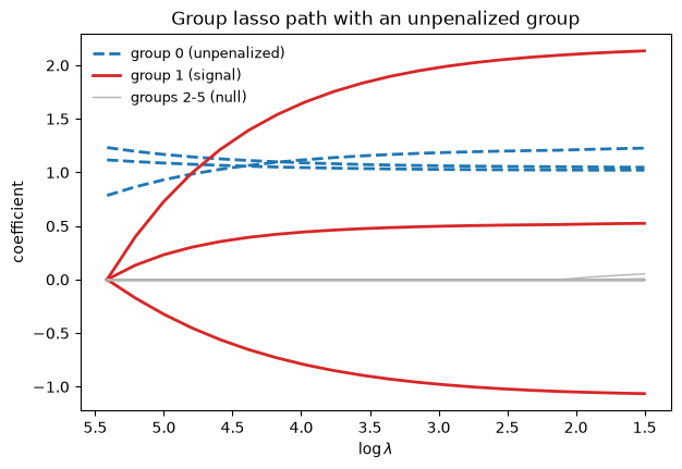
A logistic lasso path
The other losses work the same way. To include an intercept, add a column of ones and give it weight 0.
rng = np.random.default_rng(2)
n, p = 200, 20
X = rng.standard_normal((n, p))
eta = X[:, :3] @ np.array([1.5, -1, 1])
Yb = (rng.uniform(size=n) < 1 / (1 + np.exp(-eta))).astype(float)

X1 = np.column_stack([np.ones(n), X])
w = np.ones(p + 1)
w[0] = 0
enet_param = (w > 0).astype(float)
lpath = lasso.logistic(X1, Yb, w, elastic_net_param=enet_param)

# the null solution is the intercept-only fit: logit of the success proportion
print(lpath.solution[0], np.log(Yb.mean() / (1 - Yb.mean())))
np.testing.assert_allclose(lpath.solution[0], np.log(Yb.mean() / (1 - Yb.mean())), atol=1e-4)
-0.08004333775520663 -0.0800427076735365
lagrange_l = default_lagrange_sequence(lpath.penalty, lpath.grad_solution,
                                       lagrange_proportion=0.02, nstep=20)
res = strong_rules(lpath, lagrange_l, (lpath.solution.copy(), lpath.grad_solution.copy()),
                   inner_tol=1e-10)
B_l = res['beta']
print('fraction of deviance explained at smallest lambda: %.3f' % res['dev explained'])

pen = rr.weighted_l1norm(w, lagrange=lagrange_l[-1])
direct = rr.simple_problem(rr.glm.logistic(X1, Yb), pen).solve(tol=1e-13, min_its=500)
print('logistic, max |path - direct| = %.2e' % np.fabs(B_l[-1] - direct).max())
np.testing.assert_allclose(B_l[-1], direct, atol=1e-6)
fraction of deviance explained at smallest lambda: 0.352
logistic, max |path - direct| = 3.18e-09
fig, ax = plt.subplots(figsize=(7, 4.5))
loglam = np.log(lagrange_l)
for j in range(4, p + 1):
    ax.plot(loglam, B_l[:, j], color='0.7', lw=1)
for j, c in zip(range(1, 4), colors):
    ax.plot(loglam, B_l[:, j], color=c, lw=2, label=r'$\beta_{%d}$' % j)
ax.invert_xaxis()
ax.set_xlabel(r'$\log \lambda$')
ax.set_ylabel('coefficient')
ax.set_title('Logistic lasso path (intercept not shown)')
ax.legend(frameon=False, fontsize=9);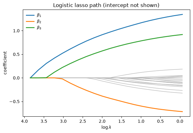
Cross-validation
cross_validate(path_obj, lagrange_seq, ...) fits the path on each training fold (by
default with strong_rules; change it with path_fitter) and scores the linear
predictor on the held-out fold. The default score is the mean squared error; pass
score=f(linpred, y) for anything else. It returns the mean and standard deviation of the
score over folds, for each .
The folds can be given as
an integer
cv: random folds drawn fromrng(a seed ornp.random.Generator);any scikit-learn splitter, e.g.
KFold(5, shuffle=True, random_state=0);an integer
cvtogether withgroup_labels, which usesGroupKFoldso that no group of cases is split across folds.
The training loss is rescaled by so that the same sequence is comparable across folds and with the full-data fit.
rng = np.random.default_rng(0)
n, p = 200, 30
X = rng.standard_normal((n, p))
beta = np.zeros(p)
beta[:5] = [3, -2, 1.5, 1, -0.5]
Y = X @ beta + rng.standard_normal(n)

path = lasso.gaussian(X, Y, np.ones(p))
lagrange = default_lagrange_sequence(path.penalty, path.grad_solution,
                                     lagrange_proportion=0.005, nstep=30)
cv_mean, cv_sd = cross_validate(path, lagrange, cv=5, rng=np.random.default_rng(3),
                                n_jobs=1, verbose=False)
imin = np.argmin(cv_mean)
print('lambda minimizing CV error: %.2f (lambda_max = %.1f), CV MSE %.3f' %
      (lagrange[imin], lagrange[0], cv_mean[imin]))
lambda minimizing CV error: 13.61 (lambda_max = 631.1), CV MSE 1.066
fig, ax = plt.subplots(figsize=(7, 4.5))
loglam = np.log(lagrange)
se = cv_sd / np.sqrt(5)
ax.fill_between(loglam, cv_mean - se, cv_mean + se, color='#1f77b4', alpha=0.2, lw=0)
ax.plot(loglam, cv_mean, color='#1f77b4', lw=2, marker='o', ms=4)
ax.axvline(loglam[imin], color='k', ls='--', lw=1)
ax.annotate(r'$\hat\lambda_{\min}$', (loglam[imin], cv_mean.max() * 0.9),
            xytext=(5, 0), textcoords='offset points')
ax.invert_xaxis()
ax.set_yscale('log')
ax.set_xlabel(r'$\log \lambda$')
ax.set_ylabel('CV mean squared error (± 1 s.e.)')
ax.set_title('5-fold cross-validation of the lasso path');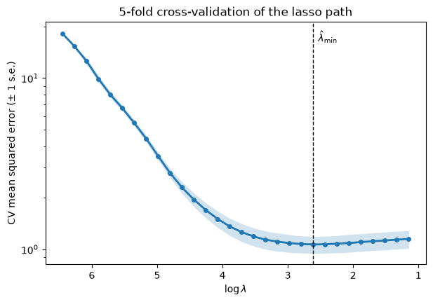
The same call with a scikit-learn splitter, and with grouped cases (say, ten cases per subject):
from sklearn.model_selection import KFold

cv_mean_kf, _ = cross_validate(path, lagrange, cv=KFold(5, shuffle=True, random_state=0),
                               n_jobs=1, verbose=False)
subjects = np.repeat(np.arange(20), 10)
cv_mean_grp, _ = cross_validate(path, lagrange, cv=5, group_labels=subjects,
                                n_jobs=1, verbose=False)
print('KFold:      lambda_min = %.2f' % lagrange[np.argmin(cv_mean_kf)])
print('GroupKFold: lambda_min = %.2f' % lagrange[np.argmin(cv_mean_grp)])
KFold: lambda_min = 16.34
GroupKFold: lambda_min = 13.61
Finally, refit at the selected : the path’s row imin is the solution there.
B = strong_rules(path, lagrange, (path.solution.copy(), path.grad_solution.copy()),
                 inner_tol=1e-10)['beta']
print('selected variables:', np.nonzero(B[imin])[0])
print('estimates:', np.round(B[imin][B[imin] != 0], 2))
selected variables: [ 0 1 2 3 4 7 20 22 23 27]
estimates: [ 3.03 -1.95 1.33 0.88 -0.36 0.04 0.01 0.01 0.02 0.14]