Many structured estimators are a smooth loss plus a penalty or constraint
applied not to itself but to a linear image : the fused lasso
penalizes differences, isotonic regression constrains them to be
nonnegative, an equality constraint pins down . This page covers
the cone constraints in regreg, the affine transforms in regreg.affine,
how atoms are composed with linear maps, and how problems with several such
terms are solved.
import numpy as np
import matplotlib.pyplot as plt
from scipy import sparse
from scipy.optimize import nnls

import regreg.api as rr
Cone constraints
A convex cone gives the constraint , represented by its
indicator function , which is 0 on and off it.
The proximal map of is Euclidean projection onto , and the
conjugate of is the indicator of the polar cone
.
regreg has
| atom | constraint | conjugate |
|---|---|---|
rr.nonnegative(p) | nonpositive | |
rr.nonpositive(p) | nonnegative | |
rr.zero_constraint(p) | zero (the zero function) | |
rr.zero(p) | none (the function 0) | zero_constraint |
rr.l2_epigraph(p+1) | l2_epigraph_polar | |
rr.l1_epigraph(p+1) | l1_epigraph_polar | |
rr.linf_epigraph(p+1) | linf_epigraph_polar |
For the epigraph cones the last coordinate holds the bound on the norm of the other coordinates.
pos = rr.nonnegative(5)
print(pos.conjugate)
print(rr.zero_constraint(5).conjugate)
print(rr.l2_epigraph(5).conjugate)
nonpositive((5,), offset=None)
zero((5,), offset=None)
l2_epigraph_polar((5,), offset=None)
Projection is proximal with a quadratic ,
written rr.identity_quadratic(1, x, 0, 0). Moreau’s decomposition says
with the two pieces orthogonal; we check this
for the second-order cone.
rng = np.random.default_rng(0)
x = rng.standard_normal(6)

K = rr.l2_epigraph(6)
Kpolar = K.conjugate
q = rr.identity_quadratic(1, x, 0, 0)
pK, pKpolar = K.proximal(q), Kpolar.proximal(q)

print('in K:      ', np.linalg.norm(pK[:-1]) <= pK[-1] + 1e-12)
np.testing.assert_allclose(pK + pKpolar, x, atol=1e-12)
np.testing.assert_allclose(pK @ pKpolar, 0, atol=1e-12)
in K: True
Nonnegative least squares
A cone constraint is an atom like any other, so nonnegative least squares,
is a simple_problem whose proximal step is the projection
. We compare it with the active-set solver
scipy.optimize.nnls.
rng = np.random.default_rng(1)
n, p = 100, 20
X = rng.standard_normal((n, p))
beta = np.zeros(p)
beta[:5] = 2
Y = X @ beta + rng.standard_normal(n)

loss = rr.squared_error(X, Y)
nnls_problem = rr.simple_problem(loss, rr.nonnegative(p))
beta_rr = nnls_problem.solve(tol=1e-12, min_its=50)

beta_scipy, _ = nnls(X, Y)
print('number of zeros:', (beta_rr == 0).sum())
print('max |regreg - scipy|:', np.abs(beta_rr - beta_scipy).max())
np.testing.assert_allclose(beta_rr, beta_scipy, atol=1e-6)
number of zeros: 8
max |regreg - scipy|: 2.1915620984636064e-09
Affine transforms
Everything in regreg.affine implements the same small interface for a map
: linear_map(x) computes , affine_map(x)
computes , adjoint_map(u) computes , and the attributes
input_shape, output_shape and affine_offset describe it. The linear
part may be a dense array, a sparse matrix or another transform, so
operators that are never formed explicitly (differences, wavelets,
convolutions) work as well as matrices.
rng = np.random.default_rng(2)
A = rng.standard_normal((4, 3))
alpha = rng.standard_normal(4)
x, u = rng.standard_normal(3), rng.standard_normal(4)

T = rr.affine_transform(A, alpha)     # x -> A x + alpha
L = rr.linear_transform(A)            # x -> A x, affine_offset is None

np.testing.assert_allclose(T.affine_map(x), A @ x + alpha)
np.testing.assert_allclose(T.linear_map(x), A @ x)
np.testing.assert_allclose(T.adjoint_map(u), A.T @ u)
print(T.input_shape, T.output_shape, L.affine_offset)
(3,) (4,) None
rr.astransform casts an array or sparse matrix to a linear_transform and
returns transforms unchanged; most functions that accept a transform call it
for you. Transforms compose with rr.affine_composition (the rightmost is
applied first), the adjoint of the linear part is T.T (an instance of
regreg.affine.adjoint), and rr.power_L estimates , the
Lipschitz constant of , by power
iteration.
B = rng.standard_normal((3, 5))
z = rng.standard_normal(5)

print(rr.astransform(A).__class__.__name__, rr.astransform(T) is T)

C = rr.affine_composition(T, rr.astransform(B))   # z -> A B z + alpha
np.testing.assert_allclose(C.affine_map(z), A @ B @ z + alpha)
np.testing.assert_allclose(T.T.linear_map(u), A.T @ u)
print('power_L:', rr.power_L(A), ' ||A||_2^2:', np.linalg.norm(A, 2)**2)
linear_transform True
power_L: 12.250354265544214 ||A||_2^2: 12.25035426578375
A selector indexes its input before (optionally) applying another
transform, which is how penalties are restricted to a subset of
coordinates.
first3 = rr.selector(slice(0, 3), (6,))
print(first3.linear_map(np.arange(6.)))
print(first3.adjoint_map(np.ones(3)))
[0. 1. 2.]
[1. 1. 1. 0. 0. 0.]
Composing atoms with linear maps
Every atom class has two constructors that compose it with a transform:
atom.linear(D, ...) represents and
atom.affine(D, alpha, ...) represents . The
remaining arguments (lagrange= or bound=) are those of the atom. Thus
is rr.l1norm.linear(D, lagrange=lam), the
constraint is rr.nonnegative.linear(D), and the equality
constraint is rr.zero_constraint.affine(A, -c).
D = np.diff(np.identity(4), axis=0)    # rows e_{i+1} - e_i
print(rr.l1norm.linear(D, lagrange=2.))
print(type(rr.nonnegative.linear(D)).__name__)
affine_atom(l1norm((3,), lagrange=2.000000, offset=None), array([[-1., 1., 0., 0.],
[ 0., -1., 1., 0.],
[ 0., 0., -1., 1.]]))
affine_cone
The proximal map of is not available in closed form, so
these composed atoms are used inside a rr.container, which takes a smooth
loss and any number of nonsmooth terms. The proximal step of a container is
computed by solving its dual, in which each composed atom contributes a dual
variable with constraint or penalty and the
transforms enter only through and (see the
solvers page).
As a first example, least squares under an equality constraint has a closed-form solution from the KKT system $$
$$
rng = np.random.default_rng(3)
n, p, m = 50, 10, 3
X = rng.standard_normal((n, p))
Y = rng.standard_normal(n)
A = rng.standard_normal((m, p))
c = rng.standard_normal(m)

problem = rr.container(rr.squared_error(X, Y), rr.zero_constraint.affine(A, -c))
# FISTA starts at beta = 0, which is infeasible (objective +inf), so the
# first relative change in objective is inf / inf; silence numpy's warning
with np.errstate(invalid='ignore'):
    beta_eq = problem.solve(tol=1e-12)

KKT = np.block([[X.T @ X, A.T], [A, np.zeros((m, m))]])
beta_kkt = np.linalg.solve(KKT, np.r_[X.T @ Y, c])[:p]
print('max |A beta - c|:', np.abs(A @ beta_eq - c).max())
print('max |regreg - KKT|:', np.abs(beta_eq - beta_kkt).max())
np.testing.assert_allclose(beta_eq, beta_kkt, atol=1e-5)
max |A beta - c|: 2.9814906099545624e-09
max |regreg - KKT|: 6.237207900855468e-07
The fused lasso and total-variation denoising
For a signal observed along a line, total-variation denoising (the one-dimensional fused lasso signal approximator) solves
that is, with the first-difference
matrix. regreg.affine.fused_lasso.difference_transform(x, order=k)
returns the sparse matrix of -th order divided differences on sorted
knots (for equally spaced knots and this is just
); trend_filter(x, order=k) wraps the same
operator as a transform for trend filtering.
from regreg.affine.fused_lasso import difference_transform, trend_filter

rng = np.random.default_rng(4)
n = 500
signal = np.zeros(n)
signal[100:150] = 7
signal[250:300] = 14
Y = signal + rng.standard_normal(n)

D = difference_transform(np.arange(n))
print(type(D).__name__, D.shape)
print(trend_filter.grid(n, order=2).output_shape)

lam = 15.
loss = rr.signal_approximator(Y)            # (1/2) ||beta - Y||^2
fused = rr.l1norm.linear(D, lagrange=lam)
tv_problem = rr.container(loss, fused)
beta_tv = tv_problem.solve()
csr_matrix (499, 500)
(498,)
The dual of this problem is a box-constrained least-squares problem,
with . Solving it separately as a simple_problem
with a supnorm bound gives a lower bound on the optimal value, so the
duality gap certifies the container’s solution.
DT = sparse.csr_matrix(D.T)
dual = rr.simple_problem(rr.squared_error(DT, Y), rr.supnorm(n - 1, bound=lam))
u_hat = dual.solve(tol=1e-12, max_its=5000)

primal_value = tv_problem.objective(beta_tv)
dual_value = 0.5 * np.sum(Y**2) - 0.5 * np.sum((Y - DT @ u_hat)**2)
gap = primal_value - dual_value
print('primal %.6f  dual %.6f  relative gap %.1e' % (primal_value, dual_value,
                                                      gap / primal_value))
assert -1e-8 < gap / primal_value < 1e-6
primal 869.691045 dual 869.690616 relative gap 4.9e-07
Adding an penalty gives the sparse fused lasso. For the signal approximator its solution is the soft-thresholded total-variation solution (Friedman et al., 2007), which gives another check on a container with two nonsmooth terms. The container’s proximal map is itself computed by an inner dual solve, so the agreement is to about 10-4 rather than to machine precision, and the exact digits vary slightly across platforms; the objective values agree much more closely.
lam1 = 2.
sparse_fused = rr.container(rr.signal_approximator(Y),
                            rr.l1norm.linear(D, lagrange=lam),
                            rr.l1norm(n, lagrange=lam1))
beta_sfl = sparse_fused.solve()

soft = np.sign(beta_tv) * np.maximum(np.abs(beta_tv) - lam1, 0)
print('max |container - soft(TV)|:', np.abs(beta_sfl - soft).max())
print('relative objective gap:',
      (sparse_fused.objective(beta_sfl) - sparse_fused.objective(soft)) /
      sparse_fused.objective(soft))
np.testing.assert_allclose(beta_sfl, soft, atol=2e-3)
assert sparse_fused.objective(beta_sfl) <= sparse_fused.objective(soft) * (1 + 1e-6)
max |container - soft(TV)|: 0.0003731997063010084
relative objective gap: 8.678139891029898e-09
fig, ax = plt.subplots(figsize=(8, 4))
ax.scatter(np.arange(n), Y, s=6, c='0.6', label='$Y$')
ax.plot(signal, 'k:', lw=1, label='true signal')
ax.plot(beta_tv, lw=2, label=r'TV, $\lambda=%g$' % lam)
ax.plot(beta_sfl, lw=1.5, label=r'sparse fused, $\lambda_1=%g$' % lam1)
ax.set_xlabel('position')
ax.legend();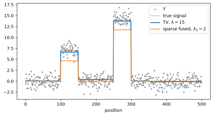
Isotonic regression
Isotonic regression is least squares under the constraint that the fit is nondecreasing, :
In regreg the constraint is rr.nonnegative.linear(D). We compare with
the pool-adjacent-violators solution from sklearn.isotonic.
from sklearn.isotonic import IsotonicRegression

rng = np.random.default_rng(5)
n = 100
x = np.arange(n)
Y = rng.standard_normal(n)
Y[:-30] += np.arange(n - 30) * 0.2

D = difference_transform(x)
iso_problem = rr.container(rr.signal_approximator(Y), rr.nonnegative.linear(D))
# the container's proximal map is itself solved iteratively, through the
# dual; by default that inner solve may stop after 5 iterations once the
# objective stops changing, which limits the accuracy here to about 1e-5
beta_iso = iso_problem.solve(tol=1e-12, max_its=5000,
                             prox_control={'min_its': 1000})

beta_pava = IsotonicRegression().fit_transform(x, Y)
print('max |regreg - sklearn|:', np.abs(beta_iso - beta_pava).max())
np.testing.assert_allclose(beta_iso, beta_pava, atol=1e-4)
max |regreg - sklearn|: 1.1800824140095756e-07
Nearly-isotonic regression
Nearly-isotonic regression (Tibshirani, Hoefling and Tibshirani, 2011) replaces the hard constraint with a penalty on decreases,
i.e. rr.positive_part.linear(-D, lagrange=lam). At the fit
is ; for large enough it is the isotonic fit.
A container builds its dual problem when it is constructed, so changing
the lagrange of one of its atoms afterwards does not change the problem
being solved (gh-104); build a new container for each value of .
neg_D = sparse.csr_matrix(-D)

fits = {}
for lam in [0.5, 2., 10., 1000.]:
    near_problem = rr.container(rr.signal_approximator(Y),
                                rr.positive_part.linear(neg_D, lagrange=lam))
    fits[lam] = near_problem.solve(tol=1e-6, max_its=5000,
                                   prox_control={'min_its': 1000}).copy()

print('max |nearly isotonic (lambda=1000) - isotonic|:',
      np.abs(fits[1000.] - beta_pava).max())
np.testing.assert_allclose(fits[1000.], beta_pava, atol=1e-4)
max |nearly isotonic (lambda=1000) - isotonic|: 9.659481037260775e-08
fig, ax = plt.subplots(figsize=(8, 4))
ax.scatter(x, Y, s=10, c='0.6', label='$Y$')
for lam in [0.5, 2., 10.]:
    ax.step(x, fits[lam], where='mid', lw=1.5, label=r'$\lambda=%g$' % lam)
ax.step(x, beta_pava, 'k--', where='mid', lw=1.5, label='isotonic')
ax.legend();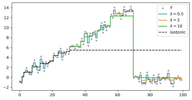
Several penalties on disjoint blocks: separable
When different penalties act on disjoint blocks of coordinates, the proximal
map splits into the proximal maps of the blocks, so no dual problem is
needed. rr.separable(shape, atoms, groups) builds such a penalty from a
list of atoms and a matching list of index objects (slices, integer arrays
or boolean masks); coordinates in no group are left unpenalized.
rr.separable_problem(loss, shape, atoms, groups) is the corresponding
simple_problem.
Here an penalty acts on the first ten coefficients and a group
( norm) penalty on the last ten. The same problem written as a
container with two selector-composed atoms, solved through the dual, gives
the same answer.
rng = np.random.default_rng(6)
n, p = 100, 20
X = rng.standard_normal((n, p))
beta = np.r_[np.ones(5), np.zeros(5), 0.3 * np.ones(5), np.zeros(5)]
Y = X @ beta + rng.standard_normal(n)

atoms = [rr.l1norm(10, lagrange=20.), rr.l2norm(10, lagrange=40.)]
groups = [slice(0, 10), slice(10, 20)]
sep_problem = rr.separable_problem(rr.squared_error(X, Y), (p,), atoms, groups)
beta_sep = sep_problem.solve(tol=1e-12, min_its=100)

as_container = rr.container(
    rr.squared_error(X, Y),
    rr.l1norm.linear(rr.selector(slice(0, 10), (p,)), lagrange=20.),
    rr.l2norm.linear(rr.selector(slice(10, 20), (p,)), lagrange=40.))
beta_cont = as_container.solve(tol=1e-11)

print(np.round(beta_sep, 3))
print('max |separable - container|:', np.abs(beta_sep - beta_cont).max())
np.testing.assert_allclose(beta_sep, beta_cont, atol=1e-5)
[ 1.035 0.737 0.865 0.693 0.685 0.072 -0. 0.067 0. -0.
0.197 0.204 0.142 0.045 0.125 0.045 -0.043 -0.037 -0.005 0.068]
max |separable - container|: 1.869700037016031e-06
The choice between the two is a matter of cost: a separable penalty has
an exact, cheap proximal map, while a container handles arbitrary
(overlapping, non-identity) linear maps at the price of an inner iterative
solve of the dual at every proximal step. That inner solve is also what
limits the container’s accuracy: here the separable solution is exact to
machine precision, while the container agrees with it to about 10-6.