Beyond the norm, regreg ships atoms for penalties that encode structure
among the coefficients: groups, feature-specific weights, sorted weights,
mixtures of these, row structure in coefficient matrices, and low rank. Each is
an atom with an exact proximal map, so each can be paired with any smooth loss
in rr.simple_problem and solved by FISTA. This page tours them with small
least-squares examples.
import numpy as np
import matplotlib.pyplot as plt
import regreg.api as rr
All examples on this page use the same simulated regression: observations, features in 10 groups of 3, and a signal in the first two groups (each of which also contains one null coefficient). The columns of have roughly unit norm, so that with noise level the noise in each score is roughly standard normal and penalty levels of a few units are natural.
rng = np.random.default_rng(0)
n, p = 200, 30
groups = np.repeat(np.arange(10), 3)
X = rng.standard_normal((n, p)) / np.sqrt(n)
beta_true = np.zeros(p)
beta_true[:6] = [8, -6, 0, 6, 0, -5]
Y = X @ beta_true + rng.standard_normal(n)

loss = rr.squared_error(X, Y)          # beta -> 1/2 ||Y - X beta||^2
The group lasso
The group lasso penalty is
where ranges over a partition of the coordinates. rr.group_lasso(groups, ...)
takes one label per coordinate; any hashable labels work. The weights are given
as a dictionary {label: w_g}; groups not in the dictionary get the default
, which makes the penalty comparable across groups of
different sizes.
gl = rr.group_lasso(groups, lagrange=1.)
print(gl.weights[0], np.sqrt(3))
print(gl.latexify())
1.7320508075688772 1.7320508075688772
\lambda_{} \sum_g w_g \|\beta[g]\|_2
The dual norm is (rr.group_lasso_dual). Evaluated at the
gradient of the loss at zero it gives , the smallest
for which .
score0 = loss.smooth_objective(np.zeros(p), mode='grad')
lagrange_max = rr.group_lasso_dual(groups, lagrange=1.).seminorm(score0)
lagrange_max7.168678034986893Fit at a fraction of :
gl = rr.group_lasso(groups, lagrange=0.3 * lagrange_max)
problem = rr.simple_problem(loss, gl)
beta_gl = problem.solve(tol=1e-12, min_its=50, max_its=5000)
group_norms = np.array([np.linalg.norm(beta_gl[groups == g]) for g in range(10)])
np.round(group_norms, 3)
array([7.885, 3.811, 0. , 0. , 0. , 0. , 0. , 0. , 0. ,
0. ])KKT conditions
minimizes if and only if, for every group,
That is, the group’s gradient lies in the dual ball of radius , on its boundary and pointing opposite to for active groups. We check both conditions:
def check_group_lasso_kkt(beta, loss, penalty, tol=1e-6):
    grad = loss.smooth_objective(beta, mode='grad')
    lam = penalty.lagrange
    for g in np.unique(penalty.groups):
        idx = penalty.groups == g
        w = penalty.weights[g]
        bg, gg = beta[idx], grad[idx]
        if w == 0:
            err = np.abs(gg).max()
            print(f'group {g}: unpenalized, max |grad_g| = {err:.1e}')
            assert err < tol
        elif np.linalg.norm(bg) > 0:
            subgrad = lam * w * bg / np.linalg.norm(bg)
            err = np.abs(-gg - subgrad).max()
            print(f'group {g}: active,   |grad_g| / (lam w_g) = '
                  f'{np.linalg.norm(gg) / (lam * w):.6f}, '
                  f'max |-grad_g - lam w_g beta_g/|beta_g|| = {err:.1e}')
            assert err < tol
        else:
            ratio = np.linalg.norm(gg) / (lam * w)
            print(f'group {g}: inactive, |grad_g| / (lam w_g) = {ratio:.6f}')
            assert ratio <= 1 + tol

check_group_lasso_kkt(beta_gl, loss, gl)
group 0: active, |grad_g| / (lam w_g) = 1.000000, max |-grad_g - lam w_g beta_g/|beta_g|| = 2.4e-12
group 1: active, |grad_g| / (lam w_g) = 1.000000, max |-grad_g - lam w_g beta_g/|beta_g|| = 4.0e-12
group 2: inactive, |grad_g| / (lam w_g) = 0.464075
group 3: inactive, |grad_g| / (lam w_g) = 0.204392
group 4: inactive, |grad_g| / (lam w_g) = 0.402718
group 5: inactive, |grad_g| / (lam w_g) = 0.437563
group 6: inactive, |grad_g| / (lam w_g) = 0.414932
group 7: inactive, |grad_g| / (lam w_g) = 0.428482
group 8: inactive, |grad_g| / (lam w_g) = 0.128011
group 9: inactive, |grad_g| / (lam w_g) = 0.840270
A solution path, warm-starting each fit from the previous one, shows groups entering the model as decreases:
lagrange_seq = lagrange_max * np.exp(np.linspace(0, np.log(0.02), 40))
path_pen = rr.group_lasso(groups, lagrange=lagrange_seq[0])
path_problem = rr.simple_problem(loss, path_pen)
path = []
for lam in lagrange_seq:
    path_pen.lagrange = lam
    path.append(path_problem.solve(tol=1e-10, min_its=20).copy())
path = np.array(path)
path_norms = np.array([[np.linalg.norm(b[groups == g]) for g in range(10)] for b in path])

fig, ax = plt.subplots(figsize=(6, 3.5))
ax.plot(lagrange_seq, path_norms)
ax.set_xscale('log')
ax.invert_xaxis()
ax.set_xlabel(r'$\lambda$')
ax.set_ylabel(r'$\|\hat\beta_g\|_2$')
ax.set_title('Group lasso path');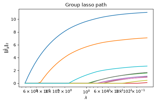
Unpenalized groups
A group with weight 0 is not penalized. This is how to always keep a block of variables (an intercept, adjustment covariates, ...) in the model. Even at , group 0 is fit, and its gradient is exactly zero (it is solved by least squares given the others):
gl0 = rr.group_lasso(groups, weights={0: 0.}, lagrange=2 * lagrange_max)
beta_gl0 = rr.simple_problem(loss, gl0).solve(tol=1e-12, min_its=50)
grad0 = loss.smooth_objective(beta_gl0, mode='grad')
print(np.round(beta_gl0[:6], 3))
print('max |gradient| on the unpenalized group:', np.abs(grad0[groups == 0]).max())
np.testing.assert_allclose(grad0[groups == 0], 0, atol=1e-6)
check_group_lasso_kkt(beta_gl0, loss, gl0)
[ 8.796 -6.902 -1.836 0. 0. 0. ]
max |gradient| on the unpenalized group: 1.0914602555089914e-12
group 0: unpenalized, max |grad_g| = 1.1e-12
group 1: inactive, |grad_g| / (lam w_g) = 0.307023
group 2: inactive, |grad_g| / (lam w_g) = 0.060595
group 3: inactive, |grad_g| / (lam w_g) = 0.047658
group 4: inactive, |grad_g| / (lam w_g) = 0.074715
group 5: inactive, |grad_g| / (lam w_g) = 0.073159
group 6: inactive, |grad_g| / (lam w_g) = 0.060755
group 7: inactive, |grad_g| / (lam w_g) = 0.070335
group 8: inactive, |grad_g| / (lam w_g) = 0.032791
group 9: inactive, |grad_g| / (lam w_g) = 0.128027
Singleton groups give the lasso
With every coordinate in its own group, and , so the group lasso is the lasso:
lam = 0.3 * np.abs(score0).max()
beta_lasso = rr.simple_problem(loss, rr.l1norm(p, lagrange=lam)).solve(tol=1e-12, min_its=50)
beta_single = rr.simple_problem(loss, rr.group_lasso(np.arange(p), lagrange=lam)).solve(tol=1e-12, min_its=50)
print('max |difference|:', np.abs(beta_lasso - beta_single).max())
np.testing.assert_allclose(beta_lasso, beta_single, atol=1e-6)
max |difference|: 8.253953076575726e-12
Sparse group lasso
The sparse group lasso adds a (weighted) term to the group penalty,
so that it selects groups and sparsifies within the selected groups.
rr.sparse_group_lasso(groups, lasso_weights, weights=..., lagrange=...) takes
the feature weights (a scalar is broadcast) in addition to the group
labels and group weights. Its proximal map is the composition of
soft-thresholding (the part) followed by group-wise shrinkage:
sgl = rr.sparse_group_lasso(groups, 0.5, lagrange=1.)
z = np.random.default_rng(1).standard_normal(p) * 3
L = 1.5
prox_sgl = sgl.lagrange_prox(z, lipschitz=L)
composed = rr.group_lasso(groups, lagrange=1.).lagrange_prox(
    rr.weighted_l1norm(0.5 * np.ones(p), lagrange=1.).lagrange_prox(z, lipschitz=L),
    lipschitz=L)
np.testing.assert_allclose(prox_sgl, composed)
print(sgl.conjugate.__class__.__name__)
sparse_group_lasso_dual
Fitted to our data, the sparse group lasso keeps the two signal groups and, unlike the group lasso fit above, also zeros the null coordinate within each of them (rows are groups):
sgl = rr.sparse_group_lasso(groups, 2.0, lagrange=1.0)
beta_sgl = rr.simple_problem(loss, sgl).solve(tol=1e-12, min_its=50)
print('group lasso:\n', np.round(beta_gl.reshape(10, 3)[:4], 3))
print('sparse group lasso:\n', np.round(beta_sgl.reshape(10, 3)[:4], 3))
print('nonzero coordinates:', np.flatnonzero(beta_sgl))
group lasso:
[[ 6.332 -4.566 -1.112]
[ 2.693 0.625 -2.623]
[ 0. 0. 0. ]
[ 0. 0. 0. ]]
sparse group lasso:
[[ 5.889 -3.885 0. ]
[ 2.29 0. -2.104]
[ 0. 0. 0. ]
[ 0. 0. 0. ]]
nonzero coordinates: [0 1 3 5]
Weighted 
rr.weighted_l1norm(weights, lagrange=λ) is with
; its dual is rr.weighted_supnorm, . Weights of
zero leave a coordinate unpenalized. A common use is the adaptive lasso, with
for a pilot estimate (here least squares):
beta_ols = np.linalg.lstsq(X, Y, rcond=None)[0]
weights = 1 / np.abs(beta_ols)
wl1 = rr.weighted_l1norm(weights, lagrange=2.)
beta_ada = rr.simple_problem(loss, wl1).solve(tol=1e-12, min_its=50)
print('nonzero:', np.flatnonzero(beta_ada))
print(np.round(beta_ada[:8], 3))
nonzero: [ 0 1 3 5 7 23 27]
[ 9.291 -5.586 -0. 5.255 0. -4.637 0. 0.521]
The conjugate is a bound-form weighted_supnorm. It is parametrized by the
reciprocal weights ( with , and when
), so the check below compares against 1 / weights:
conj = wl1.conjugate
np.testing.assert_allclose(conj.weights, 1 / weights)
u = np.random.default_rng(4).standard_normal(p)
np.testing.assert_allclose(conj.seminorm(u, lagrange=1.), np.max(np.abs(u) / weights))
print(type(conj).__module__, type(conj).__name__, conj.bound)
regreg.atoms.weighted_atoms supnorm 2.0
SLOPE
SLOPE (the sorted norm) penalizes the sorted absolute coefficients with non-increasing weights,
With the Benjamini–Hochberg-type weights
and an orthogonal design it controls the false discovery rate at level .
The penalty tends to set coefficients of similar size to exactly equal
magnitudes. Only the Lagrange form has a proximal map (computed by isotonic
regression); its conjugate is rr.slope_conjugate.
from scipy.stats import norm
q = 0.1
slope_weights = norm.ppf(1 - q * np.arange(1, p + 1) / (2 * p))
slope = rr.slope(slope_weights, lagrange=1.)
beta_slope = rr.simple_problem(loss, slope).solve(tol=1e-12, min_its=50)
print('nonzero:', np.flatnonzero(np.abs(beta_slope) > 1e-8))
print('sorted nonzero magnitudes:',
      np.sort(np.round(np.abs(beta_slope[np.abs(beta_slope) > 1e-8]), 4))[::-1])
nonzero: [ 0 1 3 5 27]
sorted nonzero magnitudes: [6.4607 3.9479 3.026 2.7468 0.6784]
A quick optimality check: for the sorted norm, is optimal iff lies in . A necessary condition, easy to check, is that the dual norm of the gradient equals when , i.e. the gradient lies on the boundary of the dual ball:
grad_slope = loss.smooth_objective(beta_slope, mode='grad')
dual_value = rr.slope_conjugate(slope_weights, lagrange=1.).seminorm(grad_slope)
print(dual_value)
np.testing.assert_allclose(dual_value, slope.lagrange, rtol=1e-5)
# and <-grad, beta> = P(beta) (the subgradient attains the support function)
np.testing.assert_allclose(-grad_slope @ beta_slope, slope.seminorm(beta_slope), rtol=1e-5)
1.0000000000000104
Mixed lasso
rr.mixed_lasso(penalty_structure, lagrange) mixes several treatments in a
single atom. penalty_structure gives one label per coordinate: the reserved
negative codes in regreg.atoms.mixed_lasso
| code | constant | treatment of |
|---|---|---|
| -1 | UNPENALIZED | no penalty |
| -2 | L1_PENALTY | |
| -3 | POSITIVE_PART | |
| -4 | NONNEGATIVE | constraint |
and every other (nonnegative) label names a group, penalized by
with weights from the weights dictionary (default
). Only the Lagrange form is available. The prox acts coordinate- or
group-wise:
from regreg.atoms.mixed_lasso import UNPENALIZED, L1_PENALTY, POSITIVE_PART, NONNEGATIVE
structure = np.array([UNPENALIZED, UNPENALIZED, L1_PENALTY, L1_PENALTY,
                      POSITIVE_PART, POSITIVE_PART, NONNEGATIVE, NONNEGATIVE, 0, 0])
ml = rr.mixed_lasso(structure, lagrange=1.)
center = np.array([3., -3., 3., -0.5, 3., -3., 3., -3., 3., 4.])
print(ml.proximal(rr.identity_quadratic(1, center, 0, 0)))
[ 3. -3. 2. 0. 2. -3.
3. 0. 2.15147186 2.86862915]
The unpenalized coordinates are untouched, the ones are soft-thresholded, the nonnegative ones are projected onto , and the group is shrunk by in norm. The positive-part coordinates are shifted down by if above it, set to 0 if in , and left unchanged if negative (the penalty is 0 there).
As a fitted example: keep the first group unpenalized, penalize the next two groups as groups, give the remaining features an penalty and constrain the last two to be nonnegative.
structure = np.array([UNPENALIZED] * 3 + [0] * 3 + [1] * 3 +
                     [L1_PENALTY] * (p - 11) + [NONNEGATIVE] * 2)
ml = rr.mixed_lasso(structure, lagrange=0.3 * lagrange_max)
beta_ml = rr.simple_problem(loss, ml).solve(tol=1e-12, min_its=50)
print(np.round(beta_ml, 3))
assert np.all(beta_ml[structure == NONNEGATIVE] >= 0)
[ 9.113 -6.427 -1.493 2.663 0.768 -2.526 0. 0. 0. 0.
0. 0. 0. 0. 0. 0. 0. 0. 0. 0.
0. 0. 0. 0. 0. 0. 0. 0.716 0.471 0.565]
Block norms for multi-response problems
For a coefficient matrix (one column per response), the block norms apply one norm to each row and combine the row norms with another:
| atom | penalty | dual |
|---|---|---|
rr.l1_l2(shape) | rr.linf_l2 | |
rr.linf_l2(shape) | rr.l1_l2 | |
rr.l1_l1(shape) | rr.linf_linf | |
rr.linf_linf(shape) | rr.l1_l1 |
rr.block_sum(atom_cls, shape) and rr.block_max(atom_cls, shape) build the
general versions for any row seminorm. l1_l2 is the multi-response (or
“multi-task”) group lasso: row collects the coefficients of feature across
responses, so a feature is selected for all responses or none. It is a group
lasso on the flattened matrix with row groups and unit weights:
q = 4
rng = np.random.default_rng(2)
Z = rng.standard_normal((p, q))
block = rr.l1_l2((p, q), lagrange=1.5)
as_group = rr.group_lasso(np.repeat(np.arange(p), q),
                          weights={i: 1. for i in range(p)}, lagrange=1.5)
np.testing.assert_allclose(block.seminorm(Z), as_group.seminorm(Z.ravel()))
np.testing.assert_allclose(block.lagrange_prox(Z), as_group.lagrange_prox(Z.ravel()).reshape(p, q))
print(block.conjugate)
linf_l2((30, 4), bound=1.500000, offset=None)
To fit a multi-response regression, the loss needs a design that acts on
matrices; rr.linear_transform(X, input_shape=(p, q)) gives the map
.
B_true = np.zeros((p, q))
B_true[:4] = rng.standard_normal((4, q)) * 4
Ymulti = X @ B_true + rng.standard_normal((n, q))
Xmap = rr.linear_transform(X, input_shape=(p, q))
loss_multi = rr.squared_error(Xmap, Ymulti)

G0 = loss_multi.smooth_objective(np.zeros((p, q)), mode='grad')
lam_max_rows = np.sqrt((G0**2).sum(1)).max()       # linf_l2 dual norm of the score
block = rr.l1_l2((p, q), lagrange=0.3 * lam_max_rows)
B_hat = rr.simple_problem(loss_multi, block).solve(tol=1e-12, min_its=50)
print('selected rows:', np.flatnonzero(np.linalg.norm(B_hat, axis=1) > 0))
selected rows: [ 0 1 2 3 15 24]
Nuclear norm and low rank
The nuclear norm is the norm of the singular values; its dual is the operator norm . The prox soft-thresholds the singular values, so penalized estimates have low rank. With the multi-response design above this is reduced-rank regression:
rng = np.random.default_rng(3)
B_lowrank = np.outer(rng.standard_normal(p), rng.standard_normal(q)) * 3   # rank 1
Ylr = X @ B_lowrank + rng.standard_normal((n, q))
loss_lr = rr.squared_error(Xmap, Ylr)

G0 = loss_lr.smooth_objective(np.zeros((p, q)), mode='grad')
lam_max_nuc = np.linalg.svd(G0, compute_uv=False)[0]   # operator norm of the score
nuc = rr.nuclear_norm((p, q), lagrange=0.3 * lam_max_nuc)
B_nuc = rr.simple_problem(loss_lr, nuc).solve(tol=1e-12, min_its=100, max_its=5000)
print('singular values of the estimate:', np.round(np.linalg.svd(B_nuc, compute_uv=False), 4))
singular values of the estimate: [16.5622 0. 0. 0. ]
The KKT conditions for the nuclear norm say that , where is the reduced SVD, , and . In particular the singular values of the gradient are at most , with exactly of them equal to :
G = loss_lr.smooth_objective(B_nuc, mode='grad')
U, D, Vt = np.linalg.svd(B_nuc)
r = (D > 1e-8).sum()
U, Vt = U[:, :r], Vt[:r]
print('rank:', r)
print('singular values of gradient / lambda:', np.round(np.linalg.svd(G, compute_uv=False) / nuc.lagrange, 6))
np.testing.assert_allclose(-U.T @ G @ Vt.T, nuc.lagrange * np.identity(r), atol=1e-5)
W = -G / nuc.lagrange - U @ Vt
assert np.linalg.svd(W, compute_uv=False)[0] <= 1 + 1e-5
rank: 1
singular values of gradient / lambda: [1. 0.858565 0.555414 0.472301]
The same atom gives matrix completion when the loss only involves the observed entries, e.g. .