The LASSO is the prototypical problem regreg is built for:
The objective splits into a smooth part (the loss, whose gradient we can
evaluate) and a nonsmooth part (the penalty, whose proximal map we can
evaluate). regreg represents each part by an object and hands the pair to a
proximal gradient solver (FISTA). This page walks through each piece and checks
the answer against first-order optimality conditions and against
scikit-learn.
import numpy as np
import regreg.api as rr

rng = np.random.default_rng(0)
n, p = 100, 20
X = rng.standard_normal((n, p))
beta_true = np.zeros(p)
beta_true[:4] = [3, -2, 1.5, 1]
Y = X @ beta_true + rng.standard_normal(n)
The loss
rr.squared_error(X, Y) is the function .
It is a smooth atom (the quadratic )
composed with the linear map .
loss = rr.squared_error(X, Y)
print(type(loss).__name__, loss.shape)
affine_smooth (20,)
Every smooth object exposes smooth_objective(beta, mode), which returns the
value (mode='func'), the gradient (mode='grad') or both (mode='both').
The solver calls only this method, so any function implementing it can be used
as a loss.
beta0 = np.zeros(p)
value = loss.smooth_objective(beta0, mode='func')
grad = loss.smooth_objective(beta0, mode='grad')
value_both, grad_both = loss.smooth_objective(beta0, mode='both')

np.testing.assert_allclose(value, 0.5 * np.sum(Y**2))
np.testing.assert_allclose(grad, X.T @ (X @ beta0 - Y))
np.testing.assert_allclose(grad_both, grad)
valuenp.float64(739.7900938805902)The same function is available as a Gaussian GLM, rr.glm.gaussian(X, Y),
which also accepts case weights and offsets (see the losses page). Its value
and gradient coincide with squared_error.
gauss = rr.glm.gaussian(X, Y)
b = rng.standard_normal(p)
f1, g1 = loss.smooth_objective(b, 'both')
f2, g2 = gauss.smooth_objective(b, 'both')
np.testing.assert_allclose([f1], [f2])
np.testing.assert_allclose(g1, g2)
The penalty
rr.l1norm(p, lagrange=lam) is the function
on . What makes it an atom is that its proximal map,
is available in closed form: soft-thresholding at . The quadratic
term is represented by an rr.identity_quadratic(L, center, linear_term, constant), i.e. .
lam = 20.
penalty = rr.l1norm(p, lagrange=lam)

z = rng.standard_normal(p) * 30
soft = np.sign(z) * np.maximum(np.abs(z) - lam, 0)
np.testing.assert_allclose(penalty.proximal(rr.identity_quadratic(1, z, 0, 0)), soft)
penaltySolving the problem
rr.simple_problem(loss, penalty) pairs one smooth function with one atom, and
solve runs FISTA with backtracking. The main controls are tol (relative
change in objective at which to stop) and min_its/max_its. The solution is
returned and also stored in problem.coefs, which is used as the starting point
of the next call to solve.
problem = rr.simple_problem(loss, penalty)
beta_hat = problem.solve(tol=1e-12, min_its=100)
np.round(beta_hat, 3)
array([ 2.669, -1.823, 0.976, 0.949, 0. , -0. , 0. , -0. ,
-0. , 0. , -0. , -0. , -0. , -0. , -0. , -0. ,
0. , -0. , 0. , -0. ])Checking the KKT conditions
The solution is characterized by , i.e. with ,
def check_lasso_kkt(grad, beta, lam, tol=1e-5):
    active = beta != 0
    eq_err = np.max(np.abs(grad[active] + lam * np.sign(beta[active])))
    ineq = np.max(np.abs(grad[~active])) if np.any(~active) else 0.
    print(f'active set size {active.sum()}, '
          f'max |g_j + lam sign(b_j)| on active set = {eq_err:.2e}, '
          f'max |g_j| off active set = {ineq:.3f} (lam = {lam})')
    assert eq_err < tol and ineq <= lam + tol

check_lasso_kkt(loss.smooth_objective(beta_hat, 'grad'), beta_hat, lam)
active set size 4, max |g_j + lam sign(b_j)| on active set = 9.73e-13, max |g_j| off active set = 19.559 (lam = 20.0)
The bound (constrained) form
Every seminorm atom can instead be used as a constraint. rr.l1norm(p, bound=delta)
is the indicator of the ball , and the problem
is solved the same way; the proximal map is now projection onto the ball.
The two forms trace out the same set of solutions. If solves the Lagrange form at , it solves the bound form with . Conversely, if solves the bound form (with the constraint active), the corresponding Lagrange multiplier is , read off from the KKT conditions above.
delta = np.abs(beta_hat).sum()
constraint = rr.l1norm(p, bound=delta)
beta_bound = rr.simple_problem(loss, constraint).solve(tol=1e-12, min_its=100)

print('max |beta_lagrange - beta_bound| =', np.max(np.abs(beta_hat - beta_bound)))
np.testing.assert_allclose(beta_bound, beta_hat, atol=1e-6)

lam_recovered = np.max(np.abs(loss.smooth_objective(beta_bound, 'grad')))
print('recovered lagrange parameter:', lam_recovered)
np.testing.assert_allclose(lam_recovered, lam, rtol=1e-5)
max |beta_lagrange - beta_bound| = 1.1879386363489175e-14
recovered lagrange parameter: 19.999999999999478
Duality and the conjugate
The convex conjugate of is the indicator of the
ball of radius ; more generally the conjugate of a
seminorm in Lagrange form is its dual norm in bound form, and vice versa.
regreg returns this as penalty.conjugate.
print(penalty.conjugate)
print(constraint.conjugate)
supnorm((20,), bound=20.000000, offset=None)
supnorm((20,), lagrange=6.417672, offset=None)
Fenchel duality gives the LASSO dual
whose solution is the residual . The constraint is
exactly the conjugate atom, so we can check dual feasibility with
penalty.conjugate.nonsmooth_objective(..., check_feasibility=True) (which
returns 0 inside the set and outside), and check that the duality gap
vanishes.
r = Y - X @ beta_hat
dual_constraint = penalty.conjugate
print('dual feasible:',
      dual_constraint.nonsmooth_objective(X.T @ r, check_feasibility=True) == 0)
print('scaled up residual feasible:',
      dual_constraint.nonsmooth_objective(1.01 * X.T @ r, check_feasibility=True) == 0)

primal = 0.5 * np.sum(r**2) + lam * np.abs(beta_hat).sum()
dual = Y @ r - 0.5 * np.sum(r**2)
print(f'primal value {primal:.8f}, dual value {dual:.8f}, |gap| {abs(primal - dual):.1e}')
np.testing.assert_allclose(primal, problem.objective(beta_hat))
assert abs(primal - dual) < 1e-5 * primal
dual feasible: True
scaled up residual feasible: False
primal value 185.56568727, dual value 185.56568727, |gap| 3.3e-12
(The residual sits on the boundary of the dual feasible set, since some constraints are active; scaling it by 1.01 leaves the set. The gap is zero only up to the solver tolerance, so it can come out slightly negative.)
Adding a ridge term: the elastic net
A quadratic is an identity_quadratic(kappa, 0, 0, 0).
Quadratics of this form are handled exactly inside the proximal map, so adding
one costs nothing. It can be passed to solve (it is used for that call only)
or attached to the atom (or loss) when constructing it. Both give the elastic
net
kappa = 5.
ridge = rr.identity_quadratic(kappa, 0, 0, 0)

beta_enet = problem.solve(quadratic=ridge, tol=1e-12, min_its=100)

penalty_enet = rr.l1norm(p, lagrange=lam, quadratic=ridge)
beta_enet2 = rr.simple_problem(loss, penalty_enet).solve(tol=1e-12, min_its=100)
np.testing.assert_allclose(beta_enet, beta_enet2, atol=1e-8)

# KKT: the gradient of the smooth part now includes kappa * beta
check_lasso_kkt(loss.smooth_objective(beta_enet, 'grad') + kappa * beta_enet,
                beta_enet, lam)
np.round(beta_enet, 3)
active set size 6, max |g_j + lam sign(b_j)| on active set = 4.58e-12, max |g_j| off active set = 18.191 (lam = 20.0)
array([ 2.520e+00, -1.716e+00,  8.740e-01,  9.170e-01,  0.000e+00,
       -0.000e+00,  0.000e+00,  0.000e+00, -0.000e+00, -0.000e+00,
       -0.000e+00, -0.000e+00,  0.000e+00, -0.000e+00, -0.000e+00,
       -1.000e-03, -0.000e+00, -0.000e+00,  0.000e+00, -3.200e-02])
Comparison with scikit-learn
sklearn.linear_model.Lasso minimizes
which is the regreg objective divided by , so .
Likewise ElasticNet minimizes
,
so and . We turn off the
intercept, since our problem has none.
from sklearn.linear_model import Lasso, ElasticNet

sk_lasso = Lasso(alpha=lam / n, fit_intercept=False, tol=1e-12, max_iter=100000).fit(X, Y)
print('lasso: max |regreg - sklearn| =', np.max(np.abs(sk_lasso.coef_ - beta_hat)))
np.testing.assert_allclose(sk_lasso.coef_, beta_hat, atol=1e-6)

alpha = (lam + kappa) / n
sk_enet = ElasticNet(alpha=alpha, l1_ratio=lam / (lam + kappa), fit_intercept=False,
                     tol=1e-12, max_iter=100000).fit(X, Y)
print('elastic net: max |regreg - sklearn| =', np.max(np.abs(sk_enet.coef_ - beta_enet)))
np.testing.assert_allclose(sk_enet.coef_, beta_enet, atol=1e-6)
lasso: max |regreg - sklearn| = 3.6415315207705135e-14
elastic net: max |regreg - sklearn| = 4.374278717023117e-14
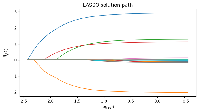
A solution path by warm starts
Solutions change continuously in , so solving over a decreasing grid
of values, starting each fit from the previous solution, is cheap.
For the solution is zero. The
lagrange attribute of the atom can be changed in place, and problem.coefs
carries the warm start from one call to the next.
import matplotlib.pyplot as plt

lam_max = np.max(np.abs(X.T @ Y))
lam_grid = lam_max * np.logspace(0, -3, 50)

path_penalty = rr.l1norm(p, lagrange=lam_max)
path_problem = rr.simple_problem(loss, path_penalty)
path = []
for l in lam_grid:
    path_penalty.lagrange = l
    path.append(path_problem.solve(tol=1e-10).copy())
path = np.array(path)

# spot check one point of the path against sklearn
k = 25
sk = Lasso(alpha=lam_grid[k] / n, fit_intercept=False, tol=1e-12, max_iter=100000).fit(X, Y)
print('path point', k, ': max |regreg - sklearn| =', np.max(np.abs(sk.coef_ - path[k])))
np.testing.assert_allclose(sk.coef_, path[k], atol=1e-5)

fig, ax = plt.subplots(figsize=(7, 4))
ax.plot(np.log10(lam_grid), path, lw=1.2)
ax.set_xlabel(r'$\log_{10} \lambda$')
ax.set_ylabel(r'$\hat\beta_j(\lambda)$')
ax.set_title('LASSO solution path')
ax.invert_xaxis()
ax.axhline(0, color='gray', lw=0.5)
plt.tight_layout()
path point 25 : max |regreg - sklearn| = 8.46136155932542e-07