Some common loss functions
There are several commonly used smooth loss functions built into
regreg:
squared error loss (
regreg.api.squared_error)Logistic loss (
regreg.glm.glm.logistic)Poisson loss (
regreg.glm.glm.poisson)Cox proportional hazards (
regreg.glm.glm.coxph, depends onstatsmodels)Huber loss (
regreg.glm.glm.huber)Huberized SVM (
regreg.smooth.losses.huberized_svm)
import numpy as np
import regreg.api as rr
import matplotlib.pyplot as plt

import rpy2.robjects as rpy2
from rpy2.robjects import numpy2ri
numpy2ri.activate()

X = np.random.standard_normal((100, 5))
X *= np.linspace(1, 3, 5)[None, :]
Y = np.random.binomial(1, 0.5, (100,))
loss = rr.glm.logistic(X, Y)
loss
rpy2.r.assign('X', X)
rpy2.r.assign('Y', Y)
r_soln = rpy2.r('glm(Y ~ X, family=binomial)$coef')
loss.solve()
np.array(r_soln)
The losses can very easily be combined with a penalty.
penalty = rr.l1norm(5, lagrange=2)
problem = rr.simple_problem(loss, penalty)
problem.solve(tol=1.e-12)
rpy2.r('''
library(glmnet)
Y = as.numeric(Y)
G = glmnet(X, Y, intercept=FALSE, standardize=FALSE, family='binomial')
print(coef(G, s=2 / nrow(X), x=X, y=Y, exact=TRUE))
''')
Suppose we want to match glmnet exactly without having to specify
intercept=FALSE and standardize=FALSE. The normalize
transformation can be used here.
n = X.shape[0]
X_intercept = np.hstack([np.ones((X.shape[0], 1)), X])
X_normalized = rr.normalize(X_intercept, intercept_column=0, scale=False)
loss_normalized = rr.glm.logistic(X_normalized, Y)
penalty_normalized = rr.weighted_l1norm([0] + [1]*5, lagrange=2.)
problem_normalized = rr.simple_problem(loss_normalized, penalty_normalized)
coefR = problem_normalized.solve(tol=1.e-12, min_its=200)
coefR
coefG = np.array(rpy2.r('as.numeric(coef(G, s=2 / nrow(X), exact=TRUE, x=X, y=Y))'))
problem_normalized.objective(coefG), problem_normalized.objective(coefR)
In theory, using the standardize=TRUE option in glmnet should be
the same as using scale=True, value=np.sqrt((n-1)/n) in
normalize, though the results don’t match without some adjustment.
This is because glmnet returns coefficients that are on the scale of
the original \(X\).
Dividing regreg’s coefficients by the col_stds corrects this.
X_intercept = np.hstack([np.ones((X.shape[0], 1)), X])
X_normalized = rr.normalize(X_intercept, intercept_column=0,
                           value=np.sqrt((n-1.)/n))
loss_normalized = rr.glm.logistic(X_normalized, Y)
penalty_normalized = rr.weighted_l1norm([0] + [1]*5, lagrange=2.)
problem_normalized = rr.simple_problem(loss_normalized, penalty_normalized)
coefR = problem_normalized.solve(min_its=300)
coefR / X_normalized.col_stds
rpy2.r('''
Y = as.numeric(Y)
G = glmnet(X, Y, standardize=TRUE, intercept=TRUE, family='binomial')
coefG = as.numeric(coef(G, s=2 / nrow(X), exact=TRUE, x=X, y=Y))
''')
coefG = np.array(rpy2.r('coefG'))
coefG = coefG * X_normalized.col_stds
problem_normalized.objective(coefG), problem_normalized.objective(coefR)
(67.64597880430388, 67.639665071862495)
Defining a new smooth function
A smooth function only really needs a smooth_objective method in
order to be used in regreg.
For example, suppose we want to define the loss
as a smooth approximation to the function
\(K=\left\{\mu: a_i^T\mu\leq b_i, 1 \leq i \leq k\right\}\) (i.e. 0 inside \(K\) and \(\infty\) outside \(K\)).
class barrier(rr.smooth_atom):

    # the argumenets [coef, offset, quadratic, initial]
    # are passed when a function is composed with a linear_transform

    objective_template = r"""\ell^{\text{barrier}}\left(%(var)s\right)\
    """

    def __init__(self,
                 shape,
                 A,
                 b,
                 coef=1.,
                 offset=None,
                 quadratic=None,
                 initial=None):
        rr.smooth_atom.__init__(self,
                                shape,
                                coef=coef,
                                offset=offset,
                                quadratic=quadratic,
                                initial=initial)
        self.A = A
        self.b = b

    def smooth_objective(self, mean_param, mode='both', check_feasibility=False):
        mean_param = self.apply_offset(mean_param)
        slack = self.b - self.A.dot(mean_param)
        if mode == 'both':
            f = self.scale(np.sum(mean_param**2/2.) - np.log(slack).sum())
            g = self.scale(mean_param + self.A.T.dot(1. / slack))
            return f, g
        elif mode == 'grad':
            g = self.scale(mean_param + self.A.T.dot(1. / slack))
            return g
        elif mode == 'func':
            f = self.scale(np.sum(mean_param**2/2.) - np.log(slack).sum())
            return f
        else:
            return ValueError('mode incorrectly specified')
A = np.array([[1, 0.], [1, 1]])
b = np.array([3., 4])
barrier_loss = barrier((2,), A, b)
barrier_loss
barrier_loss.solve(min_its=100)
The loss can now be combined with a penalty or constraint very easily.
l1_bound = rr.l1norm(2, bound=0.5)
problem = rr.simple_problem(barrier_loss, l1_bound)
problem.solve()
The loss can also be composed with a linear transform:
X = np.random.standard_normal((2,1))
lossX = rr.affine_smooth(barrier_loss, X)
lossX
lossX.solve()
Huberized lasso
The Huberized lasso minimizes the following objective
where \(H_{\delta}(\cdot)\) is a function applied element-wise,
Let’s look at the Huber loss for a smoothing parameter of \(\delta=1.2\)
q = rr.identity_quadratic(1.2, 0., 0., 0.)
loss = rr.l1norm(1, lagrange=1).smoothed(q)
xval = np.linspace(-2,2,101)
yval = [loss.smooth_objective(x, 'func') for x in xval]
huber_fig = plt.figure(figsize=(8,8))
huber_ax = huber_fig.gca()
huber_ax.plot(xval, yval)
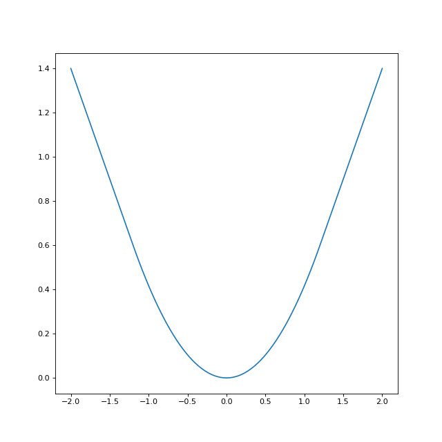
The Huber loss is built into regreg, but can also be obtained by
smoothing the l1norm atom. We will verify the two methods yield the
same solutions.
X = np.random.standard_normal((50, 10))
Y = np.random.standard_normal(50)
penalty = rr.l1norm(10,lagrange=5.)
loss_atom = rr.l1norm.affine(X, -Y, lagrange=1.).smoothed(rr.identity_quadratic(0.5,0,0,0))
loss = rr.glm.huber(X, Y, 0.5)
problem1 = rr.simple_problem(loss_atom, penalty)
print(problem1.solve(tol=1.e-12))
problem2 = rr.simple_problem(loss, penalty)
print(problem2.solve(tol=1.e-12))
Poisson regression tutorial
The Poisson regression problem minimizes the objective
which corresponds to the usual Poisson regression model
n = 100
p = 5
X = np.random.standard_normal((n,p))
Y = np.random.randint(0,100,n)
Now we can create the problem object, beginning with the loss function
loss = rr.glm.poisson(X, Y)
loss.solve()
rpy2.r.assign('Y', Y)
rpy2.r.assign('X', X)
np.array(rpy2.r('coef(glm(Y ~ X - 1, family=poisson()))'))
Logistic regression with a ridge penalty
In regreg, ridge penalties can be specified by the quadratic
attribute of a loss (or a penalty).
The regularized ridge logistic regression problem minimizes the objective
which corresponds to the usual logistic regression model
Let’s generate some sample data.
X = np.random.standard_normal((200, 10))
Y = np.random.randint(0,2,200)
Now we can create the problem object, beginning with the loss function
loss = rr.glm.logistic(X, Y)
penalty = rr.identity_quadratic(1., 0., 0., 0.)
loss.quadratic = penalty
loss
penalty.coef
1.0
loss.solve()
penalty.coef = 20.
loss.solve()
Multinomial regression
The multinomial regression problem minimizes the objective
which corresponds to a baseline category logit model for \(J\) nominal categories (e.g. Agresti, p.g. 272). For \(i \ne J\) the probabilities are measured relative to a baseline category \(J\)
from regreg.smooth.glm import multinomial_loglike
The only code needed to add multinomial regression to RegReg is a class with one method which computes the objective and its gradient.
Next, let’s generate some example data. The multinomial counts will be stored in a \(n \times J\) array
J = 5
n = 500
p = 10
X = np.random.standard_normal((n,p))
Y = np.random.randint(0,10,n*J).reshape((n,J))
Now we can create the problem object, beginning with the loss function. The coefficients will be stored in a \(p \times (J-1)\) array, and we need to let RegReg know that the coefficients will be a 2d array instead of a vector. We can do this by defining the input_shape in a linear_transform object that multiplies by X,
multX = rr.linear_transform(X, input_shape=(p,J-1))
loss = rr.multinomial_loglike.linear(multX, counts=Y)
loss.shape
Next, we can solve the problem
loss.solve()
When \(J=2\) this model should reduce to logistic regression. We can easily check that this is the case by first fitting the multinomial model
J = 2
Y = np.random.randint(0,10,n*J).reshape((n,J))
multX = rr.linear_transform(X, input_shape=(p,J-1))
loss = rr.multinomial_loglike.linear(multX, counts=Y)
solver = rr.FISTA(loss)
solver.fit(tol=1e-6)
multinomial_coefs = solver.composite.coefs.flatten()
Here is the equivalent logistic regresison model.
successes = Y[:,0]
trials = np.sum(Y, axis=1)
loss = rr.glm.logistic(X, successes, trials=trials)
solver = rr.FISTA(loss)
solver.fit(tol=1e-6)
logistic_coefs = solver.composite.coefs
Finally we can check that the two models gave the same coefficients
print(np.linalg.norm(multinomial_coefs - logistic_coefs) / np.linalg.norm(logistic_coefs))
Hinge loss
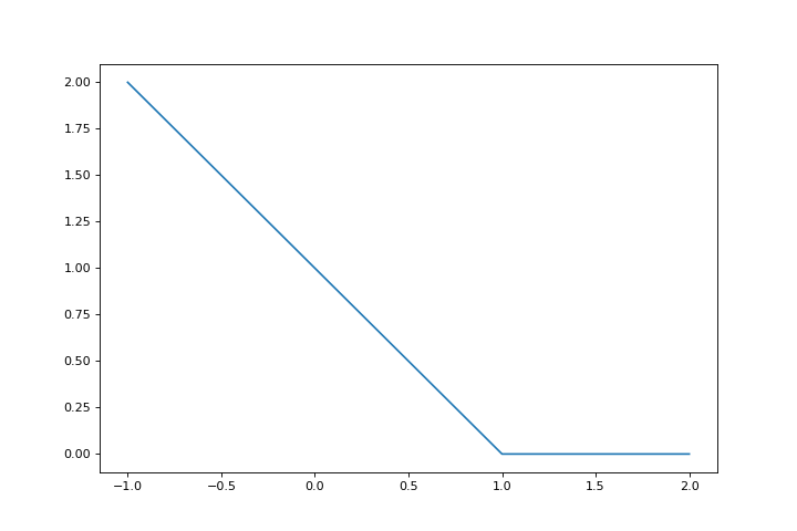
The SVM can be parametrized various ways, one way to write it as a regression problem is to use the hinge loss:
hinge = lambda x: np.maximum(1-x, 0)
fig = plt.figure(figsize=(9,6))
ax = fig.gca()
r = np.linspace(-1,2,100)
ax.plot(r, hinge(r))
The SVM loss is then
where \(Y_i \in \{-1,1\}\) and \(X_i \in \mathbb{R}^p\) is one of the feature vectors.
In regreg, the hinge loss can be represented by composition of some of the basic atoms. Specifcally, let \(g:\mathbb{R}^n \rightarrow \mathbb{R}\) be the sum of positive part function
Then,
linear_part = np.array([[-1.]])
offset = np.array([1.])
hinge_rep = rr.positive_part.affine(linear_part, offset, lagrange=1.)
hinge_rep
Let’s plot the loss to be sure it agrees with our original hinge.
ax.plot(r, [hinge_rep.nonsmooth_objective(v) for v in r])
fig
Here is a vectorized version.
N = 1000
P = 200
Y = 2 * np.random.binomial(1, 0.5, size=(N,)) - 1.
X = np.random.standard_normal((N,P))
#X[Y==1] += np.array([30,-20] + (P-2)*[0])[np.newaxis,:]
X -= X.mean(0)[np.newaxis, :]
hinge_vec = rr.positive_part.affine(-Y[:, None] * X, np.ones_like(Y), lagrange=1.)
beta = np.ones(X.shape[1])
hinge_vec.nonsmooth_objective(beta), np.maximum(1 - Y * X.dot(beta), 0).sum()
Smoothed hinge
For optimization, the hinge loss is not differentiable so it is often smoothed first.
The smoothing is applicable to general functions of the form
where \(g_{\alpha}(z) = g(z-\alpha)\) and is determined by a small quadratic term
epsilon = 0.5
smoothing_quadratic = rr.identity_quadratic(epsilon, 0, 0, 0)
smoothing_quadratic
The quadratic terms are determined by four parameters with \((C_0, x_0, v_0, c_0)\).
Smoothing of the function by the quadratic \(q\) is performed by Moreau smoothing:
where
translation by \(-\alpha\).
The basic atoms in regreg know what their conjugate is. Our hinge
loss, hinge_rep, is the composition of an atom, and an affine
transform. This affine transform is split into two pieces, the linear
part, stored as linear_transform and its offset stored as
atom.offset. It is stored with atom as atom needs knowledge
of this when computing proximal maps.
hinge_rep.atom
hinge_rep.atom.offset
hinge_rep.linear_transform.linear_operator
As we said before, hinge_rep.atom knows what its conjugate is
hinge_conj = hinge_rep.atom.conjugate
hinge_conj
The notation \(I^{\infty}\) denotes a constraint. The expression can therefore be parsed as a linear function \(\eta^T\beta\) plus the function
The term \(\eta\) is derived from hinge_rep.atom.offset and is
stored in hinge_conj.quadratic.
hinge_conj.quadratic.linear_term
Now, let’s look at the smoothed hinge loss.
smoothed_hinge_loss = hinge_rep.smoothed(smoothing_quadratic)
smoothed_hinge_loss
It is now a smooth function and its objective value and gradient can be
computed with smooth_objective.
ax.plot(r, [smoothed_hinge_loss.smooth_objective(v, 'func') for v in r])
fig
less_smooth = hinge_rep.smoothed(rr.identity_quadratic(5.e-2, 0, 0, 0))
ax.plot(r, [less_smooth.smooth_objective(v, 'func') for v in r])
fig
Fitting the SVM
We can now minimize this objective.
smoothed_vec = hinge_vec.smoothed(rr.identity_quadratic(0.2, 0, 0, 0))
soln = smoothed_vec.solve(tol=1.e-12, min_its=100)
Sparse SVM
We might want to fit a sparse version, adding a sparsifying penalty like the LASSO. This yields the problem
penalty = rr.l1norm(smoothed_vec.shape, lagrange=20)
problem = rr.simple_problem(smoothed_vec, penalty)
problem
sparse_soln = problem.solve(tol=1.e-12)
sparse_soln
What value of \(\lambda\) should we use? For the \(\ell_1\) penalty in Lagrange form, the smallest \(\lambda\) such that the solution is zero can be found by taking the dual norm, the \(\ell_{\infty}\) norm, of the gradient of the smooth part at 0.
linf_norm = penalty.conjugate
linf_norm
Just computing the conjugate will yield an \(\ell_{\infty}\) constraint, but this object can still be used to compute the desired value of \(\lambda\).
score_at_zero = smoothed_vec.smooth_objective(np.zeros(smoothed_vec.shape), 'grad')
lam_max = linf_norm.seminorm(score_at_zero, lagrange=1.)
lam_max
penalty.lagrange = lam_max * 1.001
problem.solve(tol=1.e-12, min_its=200)
penalty.lagrange = lam_max * 0.99
problem.solve(tol=1.e-12, min_its=200)
Path of solutions
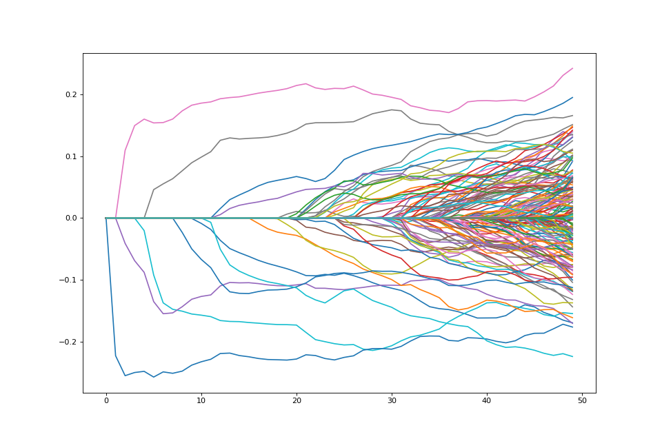
If we want a path of solutions, we can simply take multiples of
lam_max. This is similar to the strategy that packages like
glmnet use
path = []
lam_vals = (np.linspace(0.05, 1.01, 50) * lam_max)[::-1]
for lam_val in lam_vals:
    penalty.lagrange = lam_val
    path.append(problem.solve(min_its=200).copy())
fig = plt.figure(figsize=(12,8))
ax = fig.gca()
path = np.array(path)
ax.plot(path);
Changing the penalty
We may not want to penalize features the same. We may want some features to be unpenalized. This can be achieved by introducing possibly non-zero feature weights to the \(\ell_1\) norm
weights = np.random.sample(P) + 1.
weights[:5] = 0.
weighted_penalty = rr.weighted_l1norm(weights, lagrange=1.)
weighted_penalty
weighted_dual = weighted_penalty.conjugate
weighted_dual
lam_max_weight = weighted_dual.seminorm(score_at_zero, lagrange=1.)
lam_max_weight
weighted_problem = rr.simple_problem(smoothed_vec, weighted_penalty)
path = []
lam_vals = (np.linspace(0.05, 1.01, 50) * lam_max_weight)[::-1]
for lam_val in lam_vals:
    weighted_penalty.lagrange = lam_val
    path.append(weighted_problem.solve(min_its=200).copy())
fig = plt.figure(figsize=(12,8))
ax = fig.gca()
path = np.array(path)
ax.plot(path);
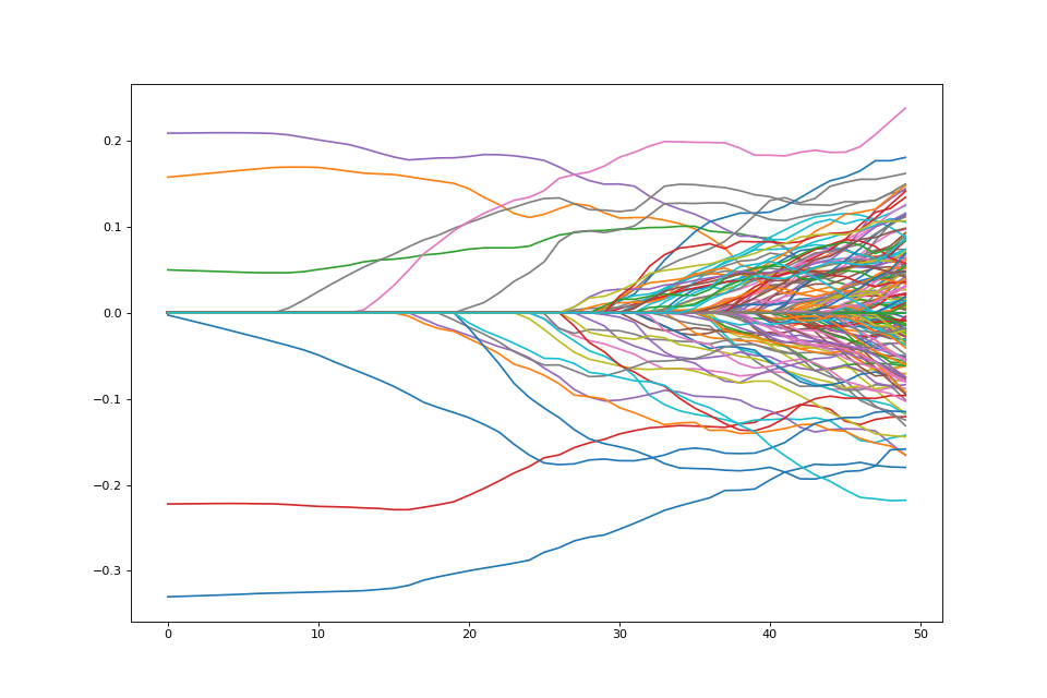
Note that there are 5 coefficients that are not penalized hence they are nonzero the entire path.
Variables may come in groups. A common penalty for this setting is the group LASSO. Let
be a partition of the set of features and \(w_g\) a weight for each group. The group LASSO penalty is
groups = []
for i in range(int(P/5)):
    groups.extend([i]*5)
weights = dict([g, np.random.sample()+1] for g in np.unique(groups))
group_penalty = rr.group_lasso(groups, weights=weights, lagrange=1.)
group_dual = group_penalty.conjugate
lam_max_group = group_dual.seminorm(score_at_zero, lagrange=1.)
group_problem = rr.simple_problem(smoothed_vec, group_penalty)
path = []
lam_vals = (np.linspace(0.05, 1.01, 50) * lam_max_group)[::-1]
for lam_val in lam_vals:
    group_penalty.lagrange = lam_val
    path.append(group_problem.solve(min_its=200).copy())
fig = plt.figure(figsize=(12,8))
ax = fig.gca()
path = np.array(path)
ax.plot(path);
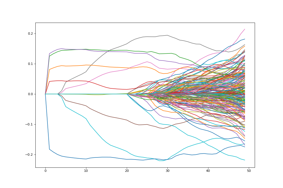
As expected, variables enter in groups here.
Bound form
The common norm atoms also have a bound form. That is, we can just as easily solve the problem
bound_l1 = rr.l1norm(P, bound=2.)
bound_l1
bound_problem = rr.simple_problem(smoothed_vec, bound_l1)
bound_problem
bound_soln = bound_problem.solve()
np.fabs(bound_soln).sum()
Support vector machine
This tutorial illustrates one version of the support vector machine, a linear example. The minimization problem for the support vector machine, following ESL is
We use the \(C\) parameterization in (12.25) of ESL
This is an example of the positive part atom combined with a smooth quadratic penalty. Above, the \(x_i\) are rows of a matrix of features and the \(y_i\) are labels coded as \(\pm 1\).
Let’s generate some data appropriate for this problem.
import numpy as np
>>>
np.random.seed(400) # for reproducibility
N = 500
P = 2
>>>
Y = 2 * np.random.binomial(1, 0.5, size=(N,)) - 1.
X = np.random.standard_normal((N,P))
X[Y==1] += np.array([3,-2])[np.newaxis,:]
X -= X.mean(0)[np.newaxis,:]
from sklearn.svm import SVC
clf = SVC(kernel='linear')
X = np.array([[-1, -1], [-2, -1], [1, 1], [2, 1]])
y = np.array([1, 1, 2, 2])
clf.fit(X, y)
print(clf.coef_, clf.dual_coef_, clf.support_)
The hinge loss is not smooth, but it can be written as the composition
of an atom (positive_part) with an affine transform determined
by the data.
Such objective functions can be smoothed. NESTA and TFOCS describe schemes in which smoothing of these atoms can be used to produce optimization problems with smooth objectives which can have additional structure imposed through optimization.
Let us try smoothing the objective and using NESTA by smoothing the hinge loss. Of course, one can also solve the usual SVC dual problem by smoothing.
def nesta_svm(X, y_pm, C=1.):
    n, p = X.shape
    X_1 = np.hstack([X, np.ones((X.shape[0], 1))])
    hinge_loss = rr.positive_part.affine(-y_pm[:,None] * X_1, + np.ones(n),
                                        lagrange=C)
    selector = np.identity(p+1)[:p]
    smooth_ = rr.quadratic_loss.linear(selector)
    soln = rr.nesta(smooth_, None, hinge_loss)
    return soln[0][:-1], soln[1]

nesta_svm(X, 2 * (y - 1.5))
Let’s try a little larger data set.
X_l = np.random.standard_normal((100, 20))
Y_l = 2 * np.random.binomial(1, 0.5, (100,)) - 1
C = 4.
clf = SVC(kernel='linear', C=C)
clf.fit(X_l, Y_l)
clf.coef_
solnR_ = nesta_svm(X_l, Y_l, C=C)[0]
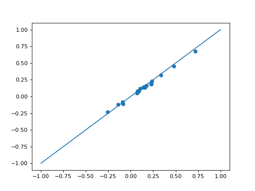
plt.scatter(clf.coef_, solnR_)
plt.plot([-1,1], [-1,1])
Using regreg, we can easily add penalty or constraint to the SVM
objective.
def nesta_svm_pen(X, y_pm, atom, C=1.):
    n, p = X.shape
    X_1 = np.hstack([X, np.ones((X.shape[0], 1))])
    hinge_loss = rr.positive_part.affine(-y_pm[:,None] * X_1, + np.ones(n),
                                        lagrange=C)
    selector = np.identity(p+1)[:p]
    smooth_ = rr.quadratic_loss.linear(selector)
    atom_sep = rr.separable((p+1,), [atom], [slice(0,p)])
    soln = rr.nesta(smooth_, atom_sep, hinge_loss)
    return soln[0][:-1]

bound = rr.l1norm(20, bound=0.8)
nesta_svm_pen(X_l, Y_l, bound)
Sparse Huberized SVM
Instead of using NESTA we can just smooth the SVM with a fixed smoothing parameter and solve the problem directly.
from regreg.smooth.losses import huberized_svm
X_l_inter = np.hstack([X_l, np.ones((X_l.shape[0],1))])
huber_svm = huberized_svm(X_l_inter, Y_l, smoothing_parameter=0.001, coef=C)
coef_h = huber_svm.solve(min_its=100)[:-1]
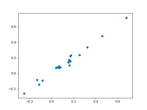
plt.scatter(coef_h, clf.coef_)
Adding penalties or constraints is again straightforward.
penalty = rr.l1norm(X_l.shape[1], lagrange=8.)
penalty_sep = rr.separable((X_l.shape[1]+1,), [penalty], [slice(0,X_l.shape[1])])
huberized_problem = rr.simple_problem(huber_svm, penalty_sep)
huberized_problem.solve()
numpy2ri.deactivate()