Using constraints

This tutorial illustrates how to use RegReg to solve problems using the container class. We illustrate with an example:

\[\frac{1}{2}||y - \beta||^{2}_{2} \ \text{subject to} \ ||D\beta||_{1} \leq \delta_1, \|\beta\|_1 \leq \delta_2\]

This problem is solved by solving a dual problem, following the general derivation in the TFOCS paper

\[ \begin{align}\begin{aligned} \frac{1}{2}||y - D^Tu_1 - u_2||^{2}_{2} + \delta_1 \|u_1\|_{\infty} + \delta_2 \|u_2\|_{\infty}\\For a general loss function, the general objective has the form\end{aligned}\end{align} \]

\[ \begin{align}\begin{aligned} {\cal L}_{\epsilon}(\beta) \ \text{subject to} \ ||D\beta||_{1} \leq \delta_1, \|\beta\|_1 \leq \delta_2\\which is solved by minimizing the dual\end{aligned}\end{align} \]

\[{\cal L}^*_{\epsilon}(-D^Tu_1-u_2) + \delta_1 \|u_1\|_{\infty} + \delta_2 \|u_2\|_{\infty}\]

Recall that for the sparse fused LASSO

\[\begin{split}D = \left(\begin{array}{rrrrrr} -1 & 1 & 0 & 0 & \cdots & 0 \\ 0 & -1 & 1 & 0 & \cdots & 0 \\ &&&&\cdots &\\ 0 &0&0&\cdots & -1 & 1 \end{array}\right)\end{split}\]

To solve this problem using RegReg we begin by loading the necessary numerical libraries

Hint

If running in the IPython console, consider running %matplotlib to enable interactive plots. If running in the Jupyter Notebook, use %matplotlib inline.

import matplotlib.pyplot as plt
import numpy as np
from scipy import sparse
import regreg.api as rr
from regreg.affine.fused_lasso import difference_transform

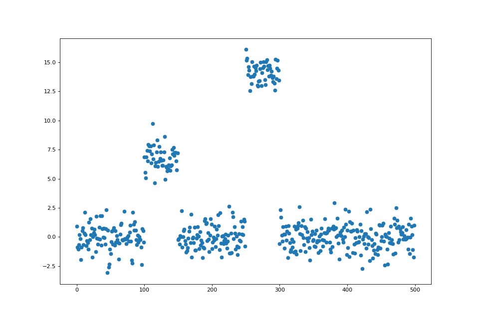
Next, let’s generate an example signal, and solve the Lagrange form of the problem

fig = plt.figure(figsize=(12,8))
ax = fig.gca()
Y = np.random.standard_normal(500); Y[100:150] += 7; Y[250:300] += 14
ax.scatter(np.arange(Y.shape[0]), Y)

(png, hires.png, pdf)

loss = rr.signal_approximator(Y)

\[\frac{C}{2}\left\|\beta - Y_{}\right\|^2_2\]

sparsity = rr.l1norm(len(Y), lagrange=1.4)
D = difference_transform(np.arange(Y.shape[0]))
fused = rr.l1norm.linear(D, lagrange=15.5)
fused

\[\lambda_{} \|X_{}\beta\|_1\]

problem = rr.dual_problem.fromprimal(loss, sparsity, fused)
problem

\[\begin{split}\begin{aligned} \text{minimize}_{\beta} & f(\beta) + g(\beta) \\ f(\beta) &= \sup_{u \in \mathbb{R}^{p} } \left[ \langle X_{1}\beta, u \rangle - \left({\cal Z}(u) + \frac{L_{1}}{2}\|u\|^2_2 + \left \langle \eta_{1}, u \right \rangle + \gamma_{1} \right) \right] \\ g(\beta) &= I^{\infty}(\|\beta[g0]\|_{\infty} \leq \delta_{0}) + I^{\infty}(\|\beta[g1]\|_{\infty} \leq \delta_{1}) \\ \end{aligned}\end{split}\]

solution = problem.solve(tol=1.e-14)

ax.plot(solution, c='yellow', linewidth=5, label='Lagrange')
fig

We will now solve this problem in constraint form, using the achieved values \(\delta_1 = \|D\widehat{\beta}\|_1, \delta_2=\|\widehat{\beta}\|_1\). By default, the container class will try to solve this problem with the two-loop strategy.

delta1 = np.fabs(D * solution).sum()
delta2 = np.fabs(solution).sum()
fused_constraint = rr.l1norm.linear(D, bound=delta1)
sparsity_constraint = rr.l1norm(Y.shape[0], bound=delta2)

constrained_problem = rr.dual_problem.fromprimal(loss,
fused_constraint, sparsity_constraint)
constrained_problem

\[\begin{split}\begin{aligned} \text{minimize}_{\beta} & f(\beta) + g(\beta) \\ f(\beta) &= \sup_{u \in \mathbb{R}^{p} } \left[ \langle X_{1}\beta, u \rangle - \left({\cal Z}(u) + \frac{L_{1}}{2}\|u\|^2_2 + \left \langle \eta_{1}, u \right \rangle + \gamma_{1} \right) \right] \\ g(\beta) &= \lambda_{0} \|\beta[g0]\|_{\infty} + \lambda_{1} \|\beta[g1]\|_{\infty} \\ \end{aligned}\end{split}\]

constrained_solution = constrained_problem.solve(tol=1.e-12)
ax.plot(constrained_solution, c='green', linewidth=3, label='Constrained')
fig

Mixing penalties and constraints

As atoms generally have both bound form and Lagrange form, we can solve problems with a mix of the two penalties. For instance, we might try minimizing this objective

\[\frac{1}{2}||y - \beta||^{2}_{2} + \lambda \|\beta\|_1 \text{ subject to} \ ||D\beta||_{1} \leq \delta.\]

mixed_problem = rr.dual_problem.fromprimal(loss, fused_constraint, sparsity)
mixed_problem

\[\begin{split}\begin{aligned} \text{minimize}_{\beta} & f(\beta) + g(\beta) \\ f(\beta) &= \sup_{u \in \mathbb{R}^{p} } \left[ \langle X_{1}\beta, u \rangle - \left({\cal Z}(u) + \frac{L_{1}}{2}\|u\|^2_2 + \left \langle \eta_{1}, u \right \rangle + \gamma_{1} \right) \right] \\ g(\beta) &= \lambda_{0} \|\beta[g0]\|_{\infty} + I^{\infty}(\|\beta[g1]\|_{\infty} \leq \delta_{1}) \\ \end{aligned}\end{split}\]

mixed_solution = mixed_problem.solve(tol=1.e-12)
ax.plot(mixed_solution, '--', linewidth=6, c='gray', label='Mixed')
ax.legend()
fig

np.fabs(D * mixed_solution).sum(), fused_constraint.atom.bound
(33.67439163971784, 33.674299924228016)

Atoms have affine offsets

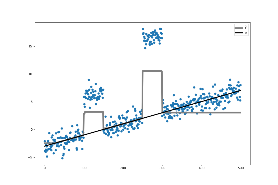
Suppose that instead of shrinking the values in the fused LASSO to 0, we want to shrink them all towards a given vector \(\alpha\)

This can be achieved, at least conceptually by minimizing

\[\frac{1}{2}||y - \beta||^{2}_{2} + \lambda_{1}||D\beta||_{1} + \lambda_2 \|\beta-\alpha\|_1\]

with

Everything is roughly the same as in the fused LASSO, we just need to change the second seminorm to have this affine offset.

Now we can create the problem object, beginning with the loss function

alpha = np.linspace(0,10,500) - 3
shrink_to_alpha = rr.l1norm(Y.shape, offset=alpha, lagrange=3.)
shrink_to_alpha

\[\lambda_{} \|\beta - \alpha_{}\|_1\]

which creates an affine_atom object with \(\lambda_2=3\). That is, it creates the penalty

\[3 \|\beta-\alpha\|_{1}\]

that will be added to a smooth loss function. Next, we create the fused lasso matrix and the associated l1norm object,

Here we first created D, converted it a sparse matrix, and then created an l1norm object with the sparse version of D and \(\lambda_1 = 25.5\). Finally, we can create the final problem object, and solve it.

loss_alpha = rr.signal_approximator(Y + alpha)
fig_alpha = plt.figure(figsize=(12,8))
ax_alpha = fig_alpha.gca()
alpha_problem = rr.dual_problem.fromprimal(loss, shrink_to_alpha, fused)
alpha_solution = alpha_problem.solve(tol=1.e-14)
ax_alpha.scatter(np.arange(Y.shape[0]), Y + alpha)
ax_alpha.plot(alpha_solution, c='gray', linewidth=5, label=r'$\hat{Y}$')
ax_alpha.plot(alpha, c='black', linewidth=3, label=r'$\alpha$')
ax_alpha.legend()

(png, hires.png, pdf)

We can then plot solution to see the result of the regression,

Atoms can be smoothed

Atoms can be smoothed using the same smoothing techniques described in NESTA and TFOCS

Recall that the sparse fused lasso minimizes the objective

\[\frac{1}{2}||y - \beta||^{2}_{2} + \lambda_{1}||D\beta||_{1} + \lambda_2 \|\beta\|_1\]

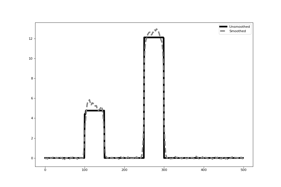
The penalty can be smoothed to create a smooth function object which can be solved with FISTA.

Q = rr.identity_quadratic(0.1, 0, 0, 0)
smoothed_sparsity = sparsity.smoothed(Q)
smoothed_sparsity

\[\sup_{u \in \mathbb{R}^{p} } \left[ \langle \beta, u \rangle - \left(I^{\infty}(\|u\|_{\infty} \leq \delta_{}) + \frac{L_{}}{2}\|u\|^2_2 \right) \right]\]

smoothed_fused = fused.smoothed(Q)

problem = rr.smooth_sum([loss, smoothed_sparsity, smoothed_fused])
solver = rr.FISTA(problem)
solver.fit(tol=1.e-10)
smooth_solution = solver.composite.coefs.copy()

smooth_fig = plt.figure(figsize=(12,8))
smooth_ax = smooth_fig.gca()
smooth_ax.plot(solution, 'k', linewidth=5, label='Unsmoothed')
smooth_ax.plot(smooth_solution, '--', c='gray', linewidth=4, label='Smoothed')
smooth_ax.legend() #doctest: +ELLIPSIS

(png, hires.png, pdf)

which has both the loss function and the seminorm represented in it. We will estimate \(\beta\) for various values of \(\epsilon\):

solns = []
for eps in [.5**i for i in range(15)]:
    Q = rr.identity_quadratic(eps, 0, 0, 0)
    smoothed_sparsity = sparsity.smoothed(Q)
    smoothed_fused = fused.smoothed(Q)
    problem = rr.smooth_sum([loss, smoothed_sparsity, smoothed_fused])
    solver = rr.FISTA(problem)
    solver.fit(tol=1.e-10)
    solns.append(solver.composite.coefs.copy())
    smooth_ax.plot(solns[-1], '--')
smooth_fig

Of course, we don’t have to smooth both atoms. We could just smooth the fused term.

smoothed_fused_constraint = fused_constraint.smoothed(rr.identity_quadratic(1e-3,0,0,0))
smooth_part = rr.smooth_sum([loss, smoothed_fused_constraint])
smoothed_constrained_problem = rr.simple_problem(smooth_part, sparsity_constraint)
smoothed_constrained_solution = smoothed_constrained_problem.solve(tol=1e-12)

ax.plot(smoothed_constrained_solution, c='black', linewidth=1, label='Smoothed')
ax.legend()
fig

Download this page as a Jupyter notebook (with outputs)